Keras and Convolutional Neural Networks (CNNs)

Creating a Convolutional Neural Network using Keras to recognize a Bulbasaur stuffed Pokemon [image source]

Today’s blog post is part two in a three-part series on building a complete end-to-end image classification + deep learning application:

• Part 1: How to (quickly) build a deep learning image dataset
• Part 2: Keras and Convolutional Neural Networks (today’s post)
• Part 3: Running a Keras model on iOS (to be published next week)

By the end of today’s blog post, you will understand how to implement, train, and evaluate a Convolutional Neural Network on your own custom dataset.

And in next week’s post, I’ll be demonstrating how you can take your trained Keras model and deploy it to a smartphone app with just a few lines of code!

To keep the series lighthearted and fun, I am fulfilling a childhood dream of mine and building a Pokedex. A Pokedex is a device that exists in the world of Pokemon, a popular TV show, video game, and trading card series (I was/still am a huge Pokemon fan).

If you are unfamiliar with Pokemon, you should think of a Pokedex as a smartphone app that can recognize Pokemon, the animal-like creatures that exist in the world of Pokemon.

You can swap in your own datasets of course, I’m just having fun and enjoying a bit of childhood nostalgia.

To learn how to train a Convolutional Neural Network with Keras and deep learning on your own custom dataset, just keep reading.

Looking for the source code to this post?
Jump right to the downloads section.

Keras and Convolutional Neural Networks

In last week’s blog post we learned how we can quickly build a deep learning image dataset — we used the procedure and code covered in the post to gather, download, and organize our images on disk.

Now that we have our images downloaded and organized, the next step is to train a Convolutional Neural Network (CNN) on top of the data.

I’ll be showing you how to train your CNN in today’s post using Keras and deep learning. The final part of this series, releasing next week, will demonstrate how you can take your trained Keras model and deploy it to a smartphone (in particular, iPhone) with only a few lines of code.

The end goal of this series is to help you build a fully functional deep learning app — use this series as an inspiration and starting point to help you build your own deep learning applications.

Let’s go ahead and get started training a CNN with Keras and deep learning.

Our deep learning dataset

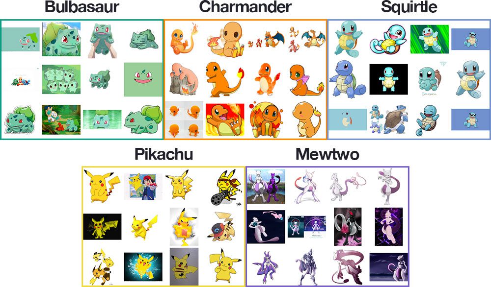
Figure 1: A montage of samples from our Pokemon deep learning dataset depicting each of the classes (i.e., Pokemon species). As we can see, the dataset is diverse, including illustrations, movie/TV show stills, action figures, toys, etc.

Our deep learning dataset consists of 1,191 images of Pokemon, (animal-like creatures that exist in the world of Pokemon, the popular TV show, video game, and trading card series).

Our goal is to train a Convolutional Neural Network using Keras and deep learning to recognize and classify each of these Pokemon.

The Pokemon we will be recognizing include:

• Bulbasaur (234 images)
• Charmander (238 images)
• Squirtle (223 images)
• Pikachu (234 images)
• Mewtwo (239 images)

A montage of the training images for each class can be seen in Figure 1 above.

As you can see, our training images include a mix of:

• Still frames from the TV show and movies
• Trading cards
• Action figures
• Toys and plushes
• Drawings and artistic renderings from fans

This diverse mix of training images will allow our CNN to recognize our five Pokemon classes across a range of images — and as we’ll see, we’ll be able to obtain 97%+ classification accuracy!

The Convolutional Neural Network and Keras project structure

Today’s project has several moving parts — to help us wrap our head around the project, let’s start by reviewing our directory structure for the project:

├── dataset
│   ├── bulbasaur [234 entries]
│   ├── charmander [238 entries]
│   ├── mewtwo [239 entries]
│   ├── pikachu [234 entries]
│   └── squirtle [223 entries]
├── examples [6 entries]
├── pyimagesearch
│   ├── __init__.py
│   └── smallervggnet.py
├── plot.png
├── lb.pickle
├── pokedex.model
├── classify.py
└── train.py

There are 3 directories:

1. dataset
   

    : Contains the five classes, each class is its own respective subdirectory to make parsing class labels easy.

2. examples
   

    : Contains images we’ll be using to test our CNN.
3. The

   pyimagesearch
   

     module: Contains our

   SmallerVGGNet
   

     model class (which we’ll be implementing later in this post).

And 5 files in the root:

1. plot.png
   

    : Our training/testing accuracy and loss plot which is generated after the training script is ran.

2. lb.pickle
   

    : Our

   LabelBinarizer
   

     serialized object file — this contains a class index to class name lookup mechamisn.

3. pokedex.model
   

    : This is our serialized Keras Convolutional Neural Network model file (i.e., the “weights file”).

4. train.py
   

    : We will use this script to train our Keras CNN, plot the accuracy/loss, and then serialize the CNN and label binarizer to disk.

5. classify.py
   

    : Our testing script.

Our Keras and CNN architecture

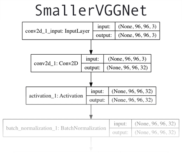
Figure 2: A VGGNet-like network that I’ve dubbed “SmallerVGGNet” will be used for training a deep learning classifier with Keras. You can find the full resolution version of this network architecture diagram here.

The CNN architecture we will be utilizing today is a smaller, more compact variant of the VGGNet network, introduced by Simonyan and Zisserman in their 2014 paper, Very Deep Convolutional Networks for Large Scale Image Recognition.

VGGNet-like architectures are characterized by:

1. Using only 3×3 convolutional layers stacked on top of each other in increasing depth
2. Reducing volume size by max pooling
3. Fully-connected layers at the end of the network prior to a softmax classifier

I assume you already have Keras installed and configured on your system. If not, here are a few links to deep learning development environment configuration tutorials I have put together:

• Configuring Ubuntu for deep learning with Python
• Setting up Ubuntu 16.04 + CUDA + GPU for deep learning with Python
• Configuring macOS for deep learning with Python

If you want to skip configuring your deep learning environment, I would recommend using one of the following pre-configured instances in the cloud:

• Amazon AMI for deep learning with Python
• Microsoft’s data science virtual machine (DSVM) for deep learning

Let’s go ahead and implement

SmallerVGGNet

 , our smaller version of VGGNet. Create a new file named

smallervggnet.py

  inside the

pyimagesearch

  module and insert the following code:

# import the necessary packages
from keras.models import Sequential
from keras.layers.normalization import BatchNormalization
from keras.layers.convolutional import Conv2D
from keras.layers.convolutional import MaxPooling2D
from keras.layers.core import Activation
from keras.layers.core import Flatten
from keras.layers.core import Dropout
from keras.layers.core import Dense
from keras import backend as K

First we import our modules — notice that they all come from Keras. Each of these are covered extensively throughout the course of reading Deep Learning for Computer Vision with Python.

Note: You’ll also want to create an

__init__.py

  file inside

pyimagesearch

  so Python knows the directory is a module. If you’re unfamiliar with

__init__.py

  files or how they are used to create modules, no worries, just use the “Downloads” section at the end of this blog post to download my directory structure, source code, and dataset + example images.

From there, we define our

SmallerVGGNet

  class:

class SmallerVGGNet:
        @staticmethod
        def build(width, height, depth, classes):
                # initialize the model along with the input shape to be
                # "channels last" and the channels dimension itself
                model = Sequential()
                inputShape = (height, width, depth)
                chanDim = -1

                # if we are using "channels first", update the input shape
                # and channels dimension
                if K.image_data_format() == "channels_first":
                        inputShape = (depth, height, width)
                        chanDim = 1

Our build method requires four parameters:

• width
  

   : The image width dimension.

• height
  

   : The image height dimension.

• depth
  

   : The depth of the image — also known as the number of channels.

• classes
  

   : The number of classes in our dataset (which will affect the last layer of our model). We’re utilizing 5 Pokemon classes in this post, but don’t forget that you could work with the 807 Pokemon species if you downloaded enough example images for each species!

Note: We’ll be working with input images that are 

96 x 96

 with a depth of

3

  (as we’ll see later in this post). Keep this in mind as we explain the spatial dimensions of the input volume as it passes through the network.

Since we’re using the TensorFlow backend, we arrange the input shape with “channels last” data ordering, but if you want to use “channels first” (Theano, etc.) then it is handled automagically on Lines 23-25.

Now, let’s start adding layers to our model:

# CONV => RELU => POOL
                model.add(Conv2D(32, (3, 3), padding="same",
                        input_shape=inputShape))
                model.add(Activation("relu"))
                model.add(BatchNormalization(axis=chanDim))
                model.add(MaxPooling2D(pool_size=(3, 3)))
                model.add(Dropout(0.25))

Above is our first 

CONV => RELU => POOL

  block.

The convolution layer has

32

  filters with a

3 x 3

  kernel. We’re using

RELU

  the activation function followed by batch normalization.

Our

POOL

  layer uses a

3 x 3

 

POOL

  size to reduce spatial dimensions quickly from

96 x 96

  to

32 x 32

 (we’ll be using  

96 x 96 x 3

 input images to train our network as we’ll see in the next section).

As you can see from the code block, we’ll also be utilizing dropout in our network architecture. Dropout works by randomly disconnecting nodes from the current layer to the next layer. This process of random disconnects during training batches helps naturally introduce redundancy into the model — no one single node in the layer is responsible for predicting a certain class, object, edge, or corner.

From there we’ll add 

(CONV => RELU) * 2

  layers before applying another

POOL

  layer:

# (CONV => RELU) * 2 => POOL
                model.add(Conv2D(64, (3, 3), padding="same",
                        input_shape=inputShape))
                model.add(Activation("relu"))
                model.add(BatchNormalization(axis=chanDim))
                model.add(Conv2D(64, (3, 3), padding="same",
                        input_shape=inputShape))
                model.add(Activation("relu"))
                model.add(BatchNormalization(axis=chanDim))
                model.add(MaxPooling2D(pool_size=(2, 2)))
                model.add(Dropout(0.25))

Stacking multiple

CONV

  and

RELU

  layers together (prior to reducing the spatial dimensions of the volume) allows us to learn a richer set of features.

Notice how:

• We’re increasing our filter size from

  32
  

    to

  64
  

   . The deeper we go in the network, the smaller the spatial dimensions of our volume, and the more filters we learn.
• We decreased how max pooling size from

  3 x 3
  

    to

  2 x 2
  

    to ensure we do not reduce our spatial dimensions too quickly.

Dropout is again performed at this stage.

Let’s add another set of  

(CONV => RELU) * 2 => POOL

 :

# (CONV => RELU) * 2 => POOL
                model.add(Conv2D(128, (3, 3), padding="same",
                        input_shape=inputShape))
                model.add(Activation("relu"))
                model.add(BatchNormalization(axis=chanDim))
                model.add(Conv2D(128, (3, 3), padding="same",
                        input_shape=inputShape))
                model.add(Activation("relu"))
                model.add(BatchNormalization(axis=chanDim))
                model.add(MaxPooling2D(pool_size=(2, 2)))
                model.add(Dropout(0.25))

Notice that we’ve increased our filter size to

128

  here. Dropout of 25% of the nodes is performed to reduce overfitting again.

And finally, we have a set of

FC => RELU

  layers and a softmax classifier:

# first (and only) set of FC => RELU layers
                model.add(Flatten())
                model.add(Dense(1024))
                model.add(Activation("relu"))
                model.add(BatchNormalization())
                model.add(Dropout(0.5))

                # softmax classifier
                model.add(Dense(classes))
                model.add(Activation("softmax"))

                # return the constructed network architecture
                return model

The fully connected layer is specified by

Dense(1024)

 with a rectified linear unit activation and batch normalization.

Dropout is performed a final time — this time notice that we’re dropping out 50% of the nodes during training. Typically you’ll use a dropout of 40-50% in our fully-connected layers and a dropout with much lower rate, normally 10-25% in previous layers (if any dropout is applied at all).

We round out the model with a softmax classifier that will return the predicted probabilities for each class label.

A visualization of the network architecture of first few layers of 

SmallerVGGNet

  can be seen in Figure 2 at the top of this section. To see the full resolution of our Keras CNN implementation of

SmallerVGGNet

 , refer to the following link.

Implementing our CNN + Keras training script

Now that

SmallerVGGNet

  is implemented, we can train our Convolutional Neural Network using Keras.

Open up a new file, name it

train.py

 , and insert the following code where we’ll import our required packages and libraries:

# set the matplotlib backend so figures can be saved in the background
import matplotlib
matplotlib.use("Agg")

# import the necessary packages
from keras.preprocessing.image import ImageDataGenerator
from keras.optimizers import Adam
from keras.preprocessing.image import img_to_array
from sklearn.preprocessing import LabelBinarizer
from sklearn.model_selection import train_test_split
from pyimagesearch.smallervggnet import SmallerVGGNet
import matplotlib.pyplot as plt
from imutils import paths
import numpy as np
import argparse
import random
import pickle
import cv2
import os

We are going to use the

"Agg"

  matplotlib backend so that figures can be saved in the background (Line 3).

The

ImageDataGenerator

  class will be used for data augmentation, a technique used to take existing images in our dataset and apply random transformations (rotations, shearing, etc.) to generate additional training data. Data augmentation helps prevent overfitting.

Line 7 imports the

Adam

  optimizer, the optimizer method used to train our network.

The

LabelBinarizer

  (Line 9) is an important class to note — this class will enable us to:

1. Input a set of class labels (i.e., strings representing the human-readable class labels in our dataset).
2. Transform our class labels into one-hot encoded vectors.
3. Allow us to take an integer class label prediction from our Keras CNN and transform it back into a human-readable label.

I often get asked hereon the PyImageSearch blog how we can transform a class label string to an integer and vice versa. Now you know the solution is to use the

LabelBinarizer

  class.

The

train_test_split

  function (Line 10) will be used to create our training and testing splits. Also take note of our

SmallerVGGNet

  import on Line 11 — this is the Keras CNN we just implemented in the previous section.

Readers of this blog are familiar with my very own imutils package. If you don’t have it installed/updated, you can install it via:

$ pip install --upgrade imutils

If you are using a Python virtual environment (as we typically do here on the PyImageSearch blog), make sure you use the

workon

  command to access your particular virtual environment before installing/upgrading

imutils

 .

From there, let’s parse our command line arguments:

# construct the argument parse and parse the arguments
ap = argparse.ArgumentParser()
ap.add_argument("-d", "--dataset", required=True,
        help="path to input dataset (i.e., directory of images)")
ap.add_argument("-m", "--model", required=True,
        help="path to output model")
ap.add_argument("-l", "--labelbin", required=True,
        help="path to output label binarizer")
ap.add_argument("-p", "--plot", type=str, default="plot.png",
        help="path to output accuracy/loss plot")
args = vars(ap.parse_args())

For our training script, we need to supply three required command line arguments:

• --dataset
  

   : The path to the input dataset. Our dataset is organized in a

  dataset
  

    directory with subdirectories representing each class. Inside each subdirectory is ~250 Pokemon images. See the project directory structure at the top of this post for more details.

• --model
  

   : The path to the output model — this training script will train the model and output it to disk.

• --labelbin
  

   : The path to the output label binarizer — as you’ll see shortly, we’ll extract the class labels from the dataset directory names and build the label binarizer.

We also have one optional argument,

--plot

 . If you don’t specify a path/filename, then a

plot.png

  file will be placed in the current working directory.

You do not need to modify Lines 22-31 to supply new file paths. The command line arguments are handled at runtime. If this doesn’t make sense to you, be sure to review my command line arguments blog post.

Now that we’ve taken care of our command line arguments, let’s initialize some important variables:

# initialize the number of epochs to train for, initial learning rate,
# batch size, and image dimensions
EPOCHS = 100
INIT_LR = 1e-3
BS = 32
IMAGE_DIMS = (96, 96, 3)

# initialize the data and labels
data = []
labels = []

# grab the image paths and randomly shuffle them
print("[INFO] loading images...")
imagePaths = sorted(list(paths.list_images(args["dataset"])))
random.seed(42)
random.shuffle(imagePaths)

Lines 35-38 initialize important variables used when training our Keras CNN:

• EPOCHS:
  

    The total number of epochs we will be training our network for (i.e., how many times our network “sees” each training example and learns patterns from it).

• INIT_LR:
  

    The initial learning rate — a value of 1e-3 is the default value for the Adam optimizer, the optimizer we will be using to train the network.

• BS:
  

    We will be passing batches of images into our network for training. There are multiple batches per epoch. The

  BS
  

    value controls the batch size.

• IMAGE_DIMS:
  

    Here we supply the spatial dimensions of our input images. We’ll require our input images to be

  96 x 96
  

    pixels with

  3
  

    channels (i.e., RGB). I’ll also note that we specifically designed SmallerVGGNet with

  96 x 96
  

    images in mind.

We also initialize two lists —

data

  and

labels

 which will hold the preprocessed images and labels, respectively.

Lines 46-48 grab all of the image paths and randomly shuffle them.

And from there, we’ll loop over each of those

imagePaths

 :

# loop over the input images
for imagePath in imagePaths:
        # load the image, pre-process it, and store it in the data list
        image = cv2.imread(imagePath)
        image = cv2.resize(image, (IMAGE_DIMS[1], IMAGE_DIMS[0]))
        image = img_to_array(image)
        data.append(image)
 
        # extract the class label from the image path and update the
        # labels list
        label = imagePath.split(os.path.sep)[-2]
        labels.append(label)

We loop over the

imagePaths

  on Line 51 and then proceed to load the image (Line 53) and resize it to accommodate our model (Line 54).

Now it’s time to update our

data

  and

labels

  lists.

We call the Keras

img_to_array

  function to convert the image to a Keras-compatible array (Line 55) followed by appending the image to our list called

data

 (Line 56).

For our

labels

  list, we extract the

label

  from the file path on Line 60 and append it (the label) on Line 61.

So, why does this class label parsing process work?

Consider that fact that we purposely created our dataset directory structure to have the following format:

dataset/{CLASS_LABEL}/{FILENAME}.jpg

Using the path separator on Line 60 we can split the path into an array and then grab the second-to-last entry in the list — the class label.

If this process seems confusing to you, I would encourage you to open up a Python shell and explore an example

imagePath

  by splitting the path on your operating system’s respective path separator.

Let’s keep moving. A few things are happening in this next code block — additional preprocessing, binarizing labels, and partitioning the data:

# scale the raw pixel intensities to the range [0, 1]
data = np.array(data, dtype="float") / 255.0
labels = np.array(labels)
print("[INFO] data matrix: {:.2f}MB".format(
        data.nbytes / (1024 * 1000.0)))

# binarize the labels
lb = LabelBinarizer()
labels = lb.fit_transform(labels)

# partition the data into training and testing splits using 80% of
# the data for training and the remaining 20% for testing
(trainX, testX, trainY, testY) = train_test_split(data,
        labels, test_size=0.2, random_state=42)

Here we first convert the

data

  array to a NumPy array and then scale the pixel intensities to the range 

[0, 1]

  (Line 64). We also convert the

labels

  from a list to a NumPy array on Line 65. An info message is printed which shows the size (in MB) of the

data

  matrix.

Then, we binarize the labels utilizing scikit-learn’s

LabelBinarizer

  (Lines 70 and 71).

With deep learning, or any machine learning for that matter, a common practice is to make a training and testing split. This is handled on Lines 75 and 76 where we create an 80/20 random split of the data.

Next, let’s create our image data augmentation object:

# construct the image generator for data augmentation
aug = ImageDataGenerator(rotation_range=25, width_shift_range=0.1,
        height_shift_range=0.1, shear_range=0.2, zoom_range=0.2,
        horizontal_flip=True, fill_mode="nearest")

Since we’re working with a limited amount of data points (< 250 images per class), we can make use of data augmentation during the training process to give our model more images (based on existing images) to train with.

Data Augmentation is a tool that should be in every deep learning practitioner’s toolbox. I cover data augmentation in the Practitioner Bundle of Deep Learning for Computer Vision with Python.

We initialize aug, our

ImageDataGenerator

 , on Lines 79-81.

From there, let’s compile the model and kick off the training:

# initialize the model
print("[INFO] compiling model...")
model = SmallerVGGNet.build(width=IMAGE_DIMS[1], height=IMAGE_DIMS[0],
        depth=IMAGE_DIMS[2], classes=len(lb.classes_))
opt = Adam(lr=INIT_LR, decay=INIT_LR / EPOCHS)
model.compile(loss="categorical_crossentropy", optimizer=opt,
        metrics=["accuracy"])

# train the network
print("[INFO] training network...")
H = model.fit_generator(
        aug.flow(trainX, trainY, batch_size=BS),
        validation_data=(testX, testY),
        steps_per_epoch=len(trainX) // BS,
        epochs=EPOCHS, verbose=1)

On Lines 85 and 86, we initialize our Keras CNN model with

96 x 96 x 3

  input spatial dimensions. I’ll state this again as I receive this question often — SmallerVGGNet was designed to accept

96 x 96 x 3

  input images. If you want to use different spatial dimensions you may need to either:

1. Reduce the depth of the network for smaller images
2. Increase the depth of the network for larger images

Do not go blindly editing the code. Consider the implications larger or smaller images will have first!

We’re going to use the

Adam

  optimizer with learning rate decay (Line 87) and then

compile

  our

model

  with categorical cross-entropy since we have > 2 classes (Lines 88 and 89).

Note: For only two classes you should use binary cross-entropy as the loss.

From there, we make a call to the Keras

fit_generator

  method to train the network (Lines 93-97). Be patient — this can take some time depending on whether you are training using a CPU or a GPU.

Once our Keras CNN has finished training, we’ll want to save both the (1) model and (2) label binarizer as we’ll need to load them from disk when we test the network on images outside of our training/testing set:

# save the model to disk
print("[INFO] serializing network...")
model.save(args["model"])

# save the label binarizer to disk
print("[INFO] serializing label binarizer...")
f = open(args["labelbin"], "wb")
f.write(pickle.dumps(lb))
f.close()

We serialize the model (Line 101) and the label binarizer (Lines 105-107) so we can easily use them later in our

classify.py

  script.

The label binarizer file contains the class index to human-readable class label dictionary. This object ensures we don’t have to hardcode our class labels in scripts that wish to use our Keras CNN.

Finally, we can plot our training and loss accuracy:

# plot the training loss and accuracy
plt.style.use("ggplot")
plt.figure()
N = EPOCHS
plt.plot(np.arange(0, N), H.history["loss"], label="train_loss")
plt.plot(np.arange(0, N), H.history["val_loss"], label="val_loss")
plt.plot(np.arange(0, N), H.history["acc"], label="train_acc")
plt.plot(np.arange(0, N), H.history["val_acc"], label="val_acc")
plt.title("Training Loss and Accuracy")
plt.xlabel("Epoch #")
plt.ylabel("Loss/Accuracy")
plt.legend(loc="upper left")
plt.savefig(args["plot"])

I elected to save my plot to disk (Line 121) rather than displaying it for two reasons: (1) I’m on a headless server in the cloud and (2) I wanted to make sure I don’t forget to save the plot.

Training our CNN with Keras

Now we’re ready to train our Pokedex CNN.

Be sure to visit the “Downloads” section of this blog post to download code + data.

Then execute the following command to train the mode; while making sure to provide the command line arguments properly:

$ $ python train.py --dataset dataset --model pokedex.model --labelbin lb.pickle
Using TensorFlow backend.
[INFO] loading images...
[INFO] data matrix: 252.07MB
[INFO] compiling model...
[INFO] training network...
name: GeForce GTX TITAN X
major: 5 minor: 2 memoryClockRate (GHz) 1.076
pciBusID 0000:09:00.0
Total memory: 11.92GiB
Free memory: 11.71GiB
Epoch 1/100
29/29 [==============================] - 2s - loss: 1.4015 - acc: 0.6088 - val_loss: 1.8745 - val_acc: 0.2134
Epoch 2/100
29/29 [==============================] - 1s - loss: 0.8578 - acc: 0.7285 - val_loss: 1.4539 - val_acc: 0.2971
Epoch 3/100
29/29 [==============================] - 1s - loss: 0.7370 - acc: 0.7809 - val_loss: 2.5955 - val_acc: 0.2008
...
Epoch 98/100
29/29 [==============================] - 1s - loss: 0.0833 - acc: 0.9702 - val_loss: 0.2064 - val_acc: 0.9540
Epoch 99/100
29/29 [==============================] - 1s - loss: 0.0678 - acc: 0.9727 - val_loss: 0.2299 - val_acc: 0.9456
Epoch 100/100
29/29 [==============================] - 1s - loss: 0.0890 - acc: 0.9684 - val_loss: 0.1955 - val_acc: 0.9707
[INFO] serializing network...
[INFO] serializing label binarizer...

Looking at the output of our training script we see that our Keras CNN obtained:

• 96.84% classification accuracy on the training set
• And 97.07% accuracy on the testing set

The training loss/accuracy plot follows:

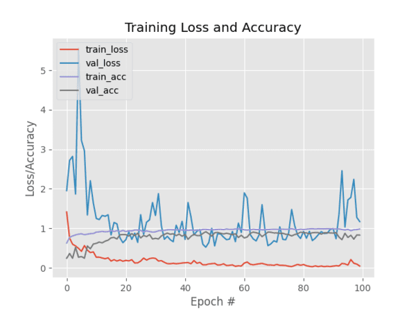
Figure 3: Training and validation loss/accuracy plot for a Pokedex deep learning classifier trained with Keras.

As you can see in Figure 3, I trained the model for 100 epochs and achieved low loss with limited overfitting. With additional training data we could obtain higher accuracy as well.

Creating our CNN and Keras testing script

Now that our CNN is trained, we need to implement a script to classify images that are not part of our training or validation/testing set. Open up a new file, name it

classify.py

 , and insert the following code:

# import the necessary packages
from keras.preprocessing.image import img_to_array
from keras.models import load_model
import numpy as np
import argparse
import imutils
import pickle
import cv2
import os

First we import the necessary packages (Lines 2-9).

From there, let’s parse command line arguments:

# construct the argument parse and parse the arguments
ap = argparse.ArgumentParser()
ap.add_argument("-m", "--model", required=True,
        help="path to trained model model")
ap.add_argument("-l", "--labelbin", required=True,
        help="path to label binarizer")
ap.add_argument("-i", "--image", required=True,
        help="path to input image")
args = vars(ap.parse_args())

We’ve have three required command line arguments we need to parse:

• --model
  

   : The path to the model that we just trained.

• --labelbin
  

   : The path to the label binarizer file.

• --image
  

   : Our input image file path.

Each of these arguments is established and parsed on Lines 12-19. Remember, you don’t need to modify these lines — I’ll show you how to run the program in the next section using the command line arguments provided at runtime.

Next, we’ll load and preprocess the image:

# load the image
image = cv2.imread(args["image"])
output = image.copy()
 
# pre-process the image for classification
image = cv2.resize(image, (96, 96))
image = image.astype("float") / 255.0
image = img_to_array(image)
image = np.expand_dims(image, axis=0)

Here we load the input 

image

  (Line 22) and make a copy called

output

  for display purposes (Line 23).

Then we preprocess the

image

  in the exact same manner that we did for training (Lines 26-29).

From there, let’s load the model + label binarizer and then classify the image:

# load the trained convolutional neural network and the label
# binarizer
print("[INFO] loading network...")
model = load_model(args["model"])
lb = pickle.loads(open(args["labelbin"], "rb").read())

# classify the input image
print("[INFO] classifying image...")
proba = model.predict(image)[0]
idx = np.argmax(proba)
label = lb.classes_[idx]

In order to classify the image, we need the

model

  and label binarizer in memory. We load both on Lines 34 and 35.

Subsequently, we classify the

image

  and create the

label

  (Lines 39-41).

The remaining code block is for display purposes:

# we'll mark our prediction as "correct" of the input image filename
# contains the predicted label text (obviously this makes the
# assumption that you have named your testing image files this way)
filename = args["image"][args["image"].rfind(os.path.sep) + 1:]
correct = "correct" if filename.rfind(label) != -1 else "incorrect"

# build the label and draw the label on the image
label = "{}: {:.2f}% ({})".format(label, proba[idx] * 100, correct)
output = imutils.resize(output, width=400)
cv2.putText(output, label, (10, 25),  cv2.FONT_HERSHEY_SIMPLEX,
        0.7, (0, 255, 0), 2)

# show the output image
print("[INFO] {}".format(label))
cv2.imshow("Output", output)
cv2.waitKey(0)

On Lines 46 and 47, we’re extracting the name of the Pokemon from the

filename

  and comparing it to the

label

 . The

correct

  variable will be either

"correct"

  or

"incorrect"

  based on this. Obviously these two lines make the assumption that your input image has a filename that contains the true label.

From there we take the following steps:

1. Append the probability percentage and

   "correct"
   

    /

   "incorrect"
   

     text to the class 

   label
   

     (Line 50).
2. Resize the

   output
   

     image so it fits our screen (Line 51).
3. Draw the

   label
   

     text on the

   output
   

     image (Lines 52 and 53).
4. Display the

   output
   

     image and wait for a keypress to exit (Lines 57 and 58).

Classifying images with our CNN and Keras

We’re now ready to run the

classify.py

  script!

Ensure that you’ve grabbed the code + images from the “Downloads” section at the bottom of this post.

Once you’ve downloaded and unzipped the archive change into the root directory of this project and follow along starting with an image of Charmander. Notice that we’ve provided three command line arguments in order to run the script:

$ python classify.py --model pokedex.model --labelbin lb.pickle \
        --image examples/charmander_counter.png
Using TensorFlow backend.
[INFO] loading network...
[INFO] classifying image...
[INFO] charmander: 99.77% (correct)

Figure 4: Correctly classifying an input image using Keras and Convolutional Neural Networks.

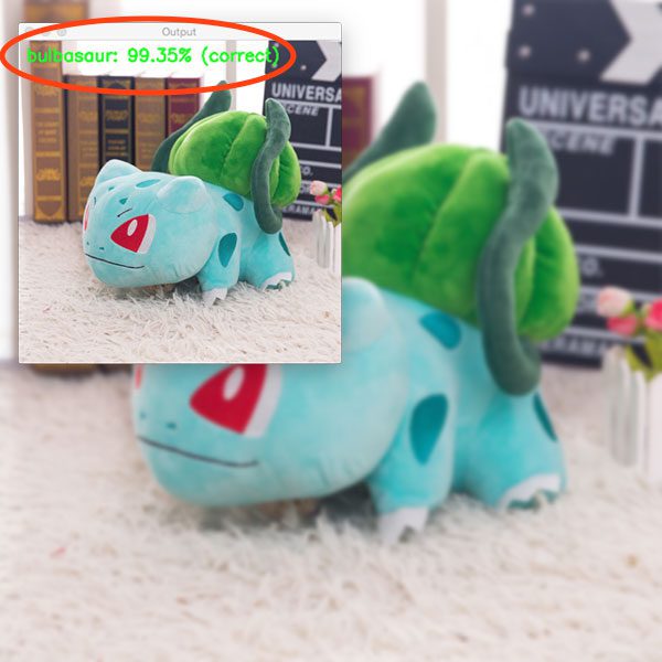
And now let’s query our model with the loyal and fierce Bulbasaur stuffed Pokemon:

$ python classify.py --model pokedex.model --labelbin lb.pickle \
        --image examples/bulbasaur_plush.png
Using TensorFlow backend.
[INFO] loading network...
[INFO] classifying image...
[INFO] bulbasaur: 99.35% (correct)

Figure 5: Again, our Keras deep learning image classifier is able to correctly classify the input image [image source]

Let’s try a toy action figure of Mewtwo (a genetically engineered Pokemon):

$ python classify.py --model pokedex.model --labelbin lb.pickle \
        --image examples/mewtwo_toy.png
Using TensorFlow backend.
[INFO] loading network...
[INFO] classifying image...
[INFO] mewtwo: 100.00% (correct)

Figure 6: Using Keras, deep learning, and Python we are able to correctly classify the input image using our CNN. [image source]

What would an example Pokedex be if it couldn’t recognize the infamous Pikachu:

$ python classify.py --model pokedex.model --labelbin lb.pickle \
        --image examples/pikachu_toy.png
Using TensorFlow backend.
[INFO] loading network...
[INFO] classifying image...
[INFO] pikachu: 99.58% (correct)

Figure 7: Using our Keras model we can recognize the iconic Pikachu Pokemon. [image source]

Let’s try the cute Squirtle Pokemon:

$ python classify.py --model pokedex.model --labelbin lb.pickle \
        --image examples/squirtle_plush.png
Using TensorFlow backend.
[INFO] loading network...
[INFO] classifying image...
[INFO] squirtle: 98.62% (correct)

Figure 8: Correctly classifying image data using Keras and a CNN. [image source]

And last but not least, let’s classify my fire-tailed Charmander again. This time he is being shy and is partially occluded by my monitor.

$ python classify.py --model pokedex.model --labelbin lb.pickle \
        --image examples/charmander_hidden.png
Using TensorFlow backend.
[INFO] loading network...
[INFO] classifying image...
[INFO] charmander: 59.82% (correct)

Figure 9: One final example of correctly classifying an input image using Keras and Convolutional Neural Networks (CNNs).

Each of these Pokemons were no match for my new Pokedex.

Currently, there are around 807 different species of Pokemon. Our classifier was trained on only five different Pokemon (for the sake of simplicity).

If you’re looking to train a classifier to recognize more Pokemon for a bigger Pokedex, you’ll need additional training images for each class. Ideally, your goal should be to have 500-1,000 images per class you wish to recognize.

To acquire training images, I suggest that you look no further than Microsoft Bing’s Image Search API. This API is hands down easier to use than the previous hack of Google Image Search that I shared (but that would work too).

Limitations of this model

One of the primary limitations of this model is the small amount of training data. I tested on various images and at times the classifications were incorrect. When this happened, I examined the input image + network more closely and found that the color(s) most dominant in the image influence the classification dramatically.

For example, lots of red and oranges in an image will likely return “Charmander” as the label. Similarly, lots of yellows in an image will normally result in a “Pikachu” label.

This is partially due to our input data. Pokemon are obviously fictitious so there no actual “real-world” images of them (other than the action figures and toy plushes).

Most of our images came from either fan illustrations or stills from the movie/TV show. And furthermore, we only had a limited amount of data for each class (~225-250 images).

Ideally, we should have at least 500-1,000 images per class when training a Convolutional Neural Network. Keep this in mind when working with your own data.

Can we use this Keras deep learning model as a REST API?

If you would like to run this model (or any other deep learning model) as a REST API, I wrote three blog posts to help you get started:

1. Building a simple Keras + deep learning REST API (Keras.io guest post)
2. A scalable Keras + deep learning REST API
3. Deep learning in production with Keras, Redis, Flask, and Apache

Summary

In today’s blog post you learned how to train a Convolutional Neural Network (CNN) using the Keras deep learning library.

Our dataset was gathered using the procedure discussed in last week’s blog post.

In particular, our dataset consists of 1,191 images of five separate Pokemon (animal-like creatures that exist in the world of Pokemon, the popular TV show, video game, and trading card series).

Using our Convolutional Neural Network and Keras, we were able to obtain 97.07% accuracy, which is quite respectable given (1) the limited size of our dataset and (2) the number of parameters in our network.

In next week’s blog post I’ll be demonstrating how we can:

1. Take our trained Keras + Convolutional Neural Network model…
2. …and deploy it to a smartphone with only a few lines of code!

It’s going to be a great post, don’t miss it!

To download the source code to this post (and be notified when next week’s can’t miss post goes live), just enter your email address in the form below!

Downloads:

If you would like to download the code and images used in this post, please enter your email address in the form below. Not only will you get a .zip of the code, I’ll also send you a FREE 11-page Resource Guide on Computer Vision and Image Search Engines, including exclusive techniques that I don’t post on this blog! Sound good? If so, enter your email address and I’ll send you the code immediately!

Email address:

The post Keras and Convolutional Neural Networks (CNNs) appeared first on PyImageSearch.

from PyImageSearch https://ift.tt/2JMPzfv
via IFTTT