Getting started with the Intel Movidius Neural Compute Stick

Let me ask you three questions:

1. What if you could could run state-of-the-art neural networks on a USB stick?
2. What if you could see over 10x performance on this USB stick compared to your CPU?
3. And what if this entire device costs under $100?

Sound interesting?

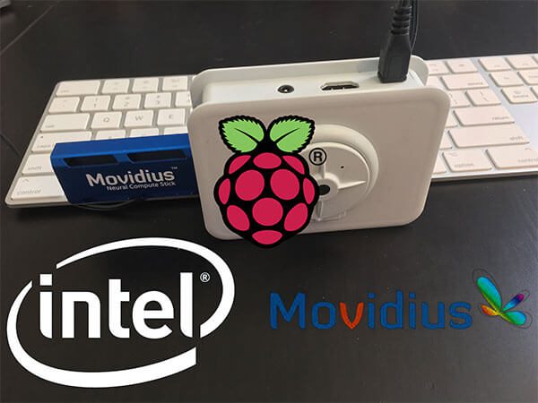
Enter Intel’s Movidius Neural Compute Stick (NCS).

Raspberry Pi users will especially welcome the device as it can dramatically improve upon image classification and object detection speeds and capabilities. You may find that the Movidius is “just what you needed” to speedup network inference time in (1) a small form factor and (2) a good price.

Inside today’s post we’ll discuss:

• What the Movidius Neural Compute Stick is capable of
• If you should buy one
• How to quickly and easily get up and running with the Movidius
• Benchmarks comparing network inference times on a MacBook Pro and Raspberry Pi

Next week I’ll provide additional benchmarks and object detection scripts using the Movidius as well.

To get started with the Intel Movidius Neural Compute Stick and to learn how you can deploy a CNN model to your Raspberry Pi + NCS, just keep reading.

Looking for the source code to this post?
Jump right to the downloads section.

Getting started with the Intel Movidius Neural Compute Stick

Today’s blog post is broken into five parts.

First, I’ll answer:

What is the Intel Movidius Neural Compute Stick and should I buy one?

From there I’ll explain the workflow of getting up and running with the Movidius Neural Compute Stick. The entire process is relatively simple, but it needs to be spelled out so that we understand how to work with the NCS

We’ll then setup our Raspberry Pi with the NCS in API-only mode. We’ll also do a quick sanity check to ensure we have communication to the NCS.

Next up, I’ll walk through my custom Raspberry Pi + Movidius NCS image classification benchmark script. We’ll be using SqueezeNet, GoogLeNet, and AlexNet.

We’ll wrap up the blog post by comparing benchmark results.

What is the Intel Movidius Neural Compute Stick?

Intel’s Neural Compute Stick is a USB-thumb-drive-sized deep learning machine.

You can think of the NCS like a USB powered GPU, although that is quite the overstatement — it is not a GPU, and it can only be used for prediction/inference, not training.

I would actually classify the NCS as a coprocessor. It’s got one purpose: running (forward-pass) neural network calculations. In our case, we’ll be using the NCS for image classification.

The NCS should not be used for training a neural network model, rather it is designed for deployable models. Since the device is meant to be used on single board computers such as the Raspberry Pi, the power draw is meant to be minimal, making it inappropriate for actually training a network.

So now you’re wondering: Should I buy the Movidius NCS?

At only $77 dollars, the NCS packs a punch. You can buy the device on Amazon or at any of the retailers listed on Intel’s site.

Under the hood of the NCS is a Myriad 2 processor (28 nm) capable of 80-150 GFLOPS performance. This processor is also known as a Vision Processing Unit (or vision accelerator) and it consumes only 1W of power (for reference, the Raspberry Pi 3 B consumes 1.2W with HDMI off, LEDs off, and WiFi on).

Whether buying the NCS is worth it to you depends on the answers to several questions:

1. Do you have an immediate use case or do you have $77 to burn on another toy?
2. Are you willing to deal with the growing pains of joining a young community? While certainly effective, we don’t know if these “vision processing units” are here to stay.
3. Are you willing to devote a machine (or VM) to the SDK?
4. Pi Users: Are you willing to devote a separate Pi or at least a separate microSD to the NCS? Are you aware that the device based on it’s form factor dimensions will block 3 USB ports unless you use a cable to go to the NCS dongle?

Question 1 is up to you.

The reason I’m asking question 2 is because Intel is notorious for poor documentation and even discontinuing their products as they did with the Intel Galileo.

I’m not suggesting that either will occur with the NCS. The NCS is in the deep learning domain which is currently heading full steam ahead, so the future of this product does look bright. It also doesn’t hurt that there aren’t too many competing products.

Questions 2 and 3 (and their answers) are related. In short, you can’t isolate the development environments with virtual environments and the installer actually removes previous installations of OpenCV from your system. For this reason you should not get the installer scripts anywhere near your current projects and working environments. I learned the hard way. Trust me.

Hopefully I haven’t scared you off — that is not my intention. Most people will be purchasing the Movidius NCS to pair with a Raspberry Pi or other single board computer.

Question 4 is for Pi users. When it comes to the Pi, if you’ve been following any other tutorials on PyImageSearch.com, you’re aware that I recommend Python virtual environments to isolate your Python projects and associated dependencies. Python virtual environments are a best practice in the Python community.

One of my biggest gripes with the Neural Compute Stick is that Intel’s install scripts will actually make your virtual environments nearly unusable. The installer downloads packages from the Debian/Ubuntu Aptitude repos and changes your PYTHONPATH system variable.

It get really messy real quick and to be on the safe side, you should use a fresh microSD (purchase a 32GB 98MB/s microSD on Amazon) with Raspbian Stretch. You might even buy another Pi to marry to the NCS if you’re working on a deployable project.

When I received my NCS I was excited to plug it into my Pi…but unfortunately I was off to a rough start.

Check out the image below.

I found out that with the NCS plugged in, it blocks all 3 other USB ports on my Pi. I can’t even plug my wireless keyboard/mouse dongle in another port!

Now, I understand that the NCS is meant to be used with devices other than the Raspberry Pi, but given that the Raspberry Pi is one of the most used single board systems, I was a bit surprised that Intel didn’t consider this — perhaps it’s because the device consumes a lot of power and they want you to think twice about plugging in additional peripherals to your Pi.

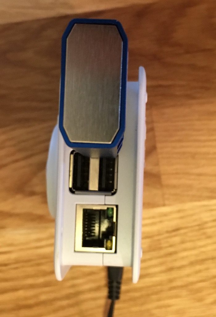
Figure 1: The Intel Movidius NCS blocks the 3 other USB ports from easy access.

This is very frustrating. The solution is to buy a 6in USB 3.0 extension such as this one:

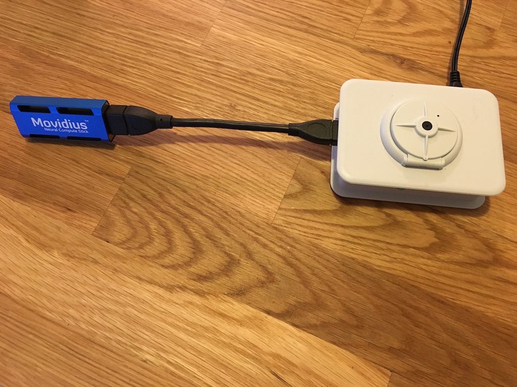
Figure 2: Using a 6in USB extension dongle with the Movidius NCS and Raspberry Pi allows access the other 3 USB ports.

With those considerations in mind, the Movidius NCS is actually a great device at a good value. So let’s dive into the workflow.

Movidius NCS Workflow

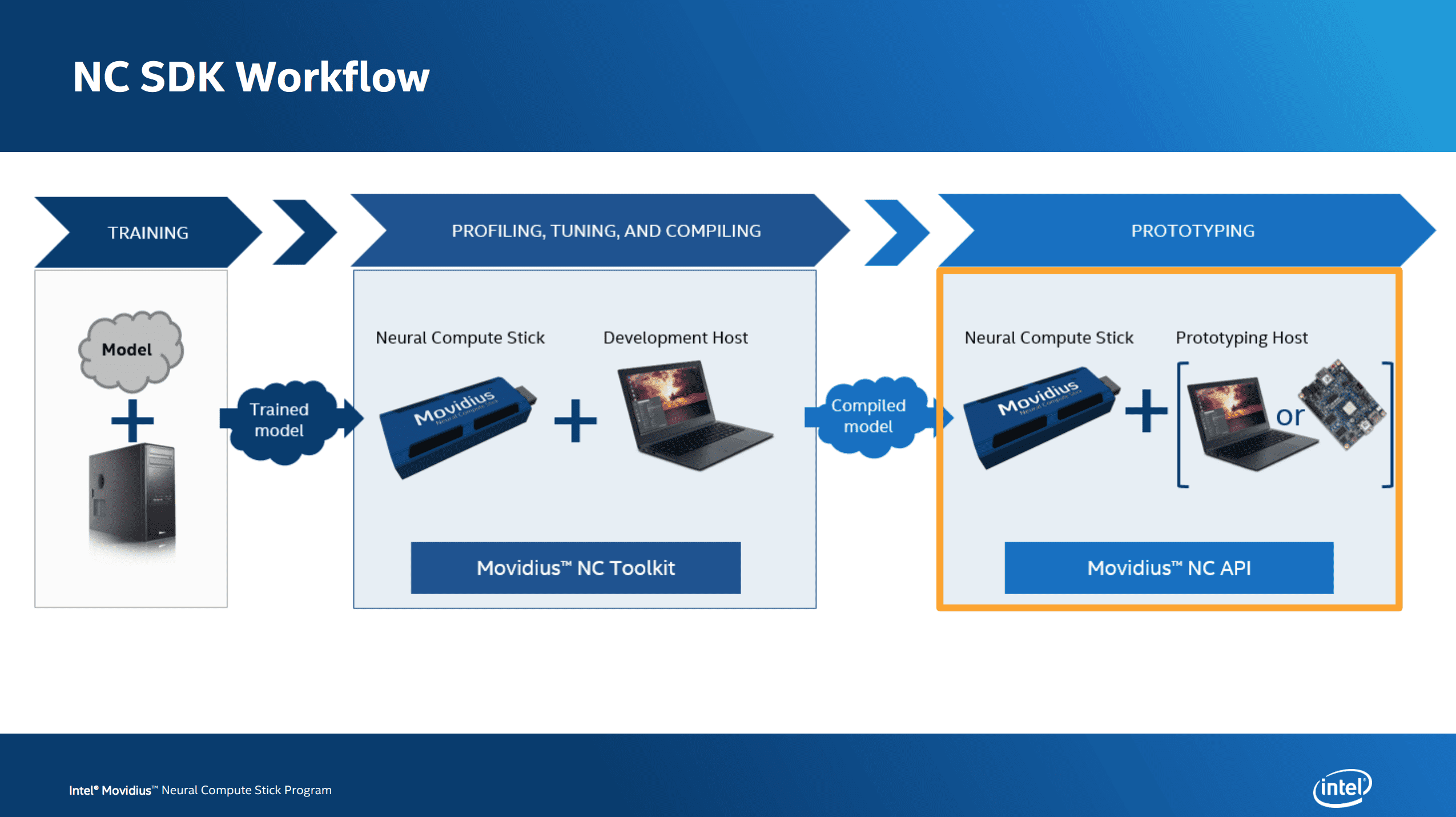
Figure 3: The Intel Movidius NCS workflow (image credit: Intel)

Working with the NCS is quite easy once you understand the workflow.

The bottom line is that you need a graph file to deploy to the NCS. This graph file can live in the same directory as your Python script if you’d like — it will get sent to the NCS using the NCS API.

In general, the workflow of using the NCS is:

1. Use a pre-trained TensorFlow/Caffe model or train a network with Tensorflow/Caffe on Ubuntu or Debian.
2. Use the NCS SDK toolchain to generate a graph file.
3. Deploy the graph file and NCS to your single board computer running a Debian flavor of Linux. I used a Raspberry Pi 3 B running Raspbian (Debian based).
4. With Python, use the NCS API to send the graph file to the NCS and request predictions on images. Process the prediction results and take an (arbitrary) action based on the results.

Today, we’ll set up the Raspberry Pi in with the NCS API-only mode toolchain. This setup also generates the bare-minimum SDK tools to create graph files. It does not install Caffe, Tensorflow, etc.

For the sake of simplicity, we’ll be using a pre-trained Caffe model and prototxt files that come from the Movidius GitHub page (indirectly a Makefile downloads them from the DeepScale GitHub repo).

Executing the Makefile will:

1. Download the Caffe files
2. Use the NCS API to generate a graph file

From there, we’ll try out the Movidius using their example script + a single static image.

Finally, we’ll create our own custom image classification benchmarking script. You’ll notice that this script is based heavily on a previous post on Deep learning with the Raspberry Pi and OpenCV.

First, let’s prepare our Raspberry Pi.

Setting up your Raspberry Pi and the NCS in API-only mode

I learned the hard way that the Raspberry Pi can’t handle the SDK (what was I thinking?) by reading some sparse documentation.

I later started from square one and found better documentation that instructed me to set up my Pi in API-only mode (now this makes sense). I was quickly up and running in this fashion and I’ll show you how to do the same thing.

For your Pi, I recommend that you install the SDK in API-only mode on a fresh installation of Raspbian Stretch.

To install the Raspbian Stretch OS on your Pi, grab the Stretch image here and then flash the card using these instructions.

From there, boot up your Pi and connect to WiFi. You can complete all of the following actions over an SSH connection or using a monitor + keyboard/mouse (with the 6inch dongle listed above as the USB ports are blocked by the NCS) if you prefer.

Let’s update the system:

$ sudo apt-get update && sudo apt-get upgrade

Then let’s install a bunch of packages:

$ sudo apt-get install -y libusb-1.0-0-dev libprotobuf-dev
$ sudo apt-get install -y libleveldb-dev libsnappy-dev
$ sudo apt-get install -y libopencv-dev
$ sudo apt-get install -y libhdf5-serial-dev protobuf-compiler
$ sudo apt-get install -y libatlas-base-dev git automake 
$ sudo apt-get install -y byacc lsb-release cmake 
$ sudo apt-get install -y libgflags-dev libgoogle-glog-dev 
$ sudo apt-get install -y liblmdb-dev swig3.0 graphviz 
$ sudo apt-get install -y libxslt-dev libxml2-dev 
$ sudo apt-get install -y gfortran 
$ sudo apt-get install -y python3-dev python-pip python3-pip 
$ sudo apt-get install -y python3-setuptools python3-markdown 
$ sudo apt-get install -y python3-pillow python3-yaml python3-pygraphviz
$ sudo apt-get install -y python3-h5py python3-nose python3-lxml 
$ sudo apt-get install -y python3-matplotlib python3-numpy 
$ sudo apt-get install -y python3-protobuf python3-dateutil 
$ sudo apt-get install -y python3-skimage python3-scipy 
$ sudo apt-get install -y python3-six python3-networkx

Notice that we’ve installed

libopencv-dev

  from the Debian repositories. This is the first time I’m ever recommending it and hopefully the last time as well. Installing OpenCV via apt-get (1) installs an older version of OpenCV, (2) does not install the full version of OpenCV, and (3) does not take advantage of various system operations. Again, I do not recommend this method to installing OpenCV.

Additionally, you can see we’re installing a whole bunch of packages that I generally prefer to manage inside Python virtual environments with pip. Be sure you are using a fresh memory card so you don’t mess up other projects that you’ve been working on, on your Pi.

From there, let’s make a workspace directory and clone the NCSDK:

$ cd ~
$ mkdir workspace
$ cd workspace
$ git clone https://github.com/movidius/ncsdk

And while we’re at it, let’s clone down the NC App Zoo as we’ll want it for later.

$ git clone https://github.com/movidius/ncappzoo

And from there, navigate into the following directory:

$ cd ncsdk/api/src

In that directory we’ll use the Makefile to install SDK in API-only mode:

$ make
$ sudo make install

Test the Raspberry Pi installation on the NCS

Let’s test the installation by using code from the NC App Zoo. Be sure that the NCS is plugged into your Pi at this point.

$ cd ncappzoo/apps/hello_ncs_py
$ make run

making run
python3 hello_ncs.py;
Hello NCS! Device opened normally.
Goodbye NCS! Device closed normally.
NCS device working.

You should see the exact output as above.

Generating your Movidius NCS neural network

SqueezeNet is included with the NC App Zoo and it is easy to generate the required graph file. The Makefile does it all for us:

$ cd ~/workspace/ncappzoo/caffe/SqueezeNet
$ make all
$ python run.py
...
------- predictions --------

     electric guitar 99.12 %
              vacuum 0.34 %
     acoustic guitar 0.15 %
           corkscrew 0.10 %
                hook 0.07 %

Classification with the Movidius NCS

If you open up the

run.py

  file that we just created with the Makefile, you’ll notice that most inputs are hardcoded and that the file is ugly in general.

Instead, we’re going to create our own file for classification and benchmarking.

In a previous post, Deep learning on the Raspberry Pi with OpenCV, I described how to use the OpenCV’s DNN module to perform object classification.

Today, we’re going to modify that exact same script to make it compatible with the Movidius NCS.

If you compare both scripts you’ll see that they are nearly identical. For this reason, I’ll simply be pointing out the differences, so I encourage you to refer to the previous post for full explanations.

Each script is included in the “Downloads” section of this blog post, so be sure to grab the zip and follow along.

Let’s review the differences in the modified file named 

pi_ncs_deep_learning.py

 :

# import the necessary packages
from mvnc import mvncapi as mvnc
import numpy as np
import argparse
import time
import cv2

Here we are importing our packages — the only difference is on Line 2 where we import the

mvncapi as mvnc

 . This import is for the NCS API.

From there, we need to parse our command line arguments:

# construct the argument parse and parse the arguments
ap = argparse.ArgumentParser()
ap.add_argument("-i", "--image", required=True,
        help="path to input image")
ap.add_argument("-g", "--graph", required=True,
        help="path to graph file")
ap.add_argument("-d", "--dim", type=int, required=True,
        help="dimension of input to network")
ap.add_argument("-l", "--labels", required=True,
        help="path to ImageNet labels (i.e., syn-sets)")
args = vars(ap.parse_args())

In this block I’ve removed two arguments (

--prototxt

  and

--model

 ) while adding two arguments (

--graph

  and

--dim

 ).

The

--graph

  argument is the path to our graph file — it takes the place of the prototxt and model.

Graph files can be generated via the NCS SDK, which we’ll cover in next week’s blog post. I’ve included the graph files for this week in the “Downloads“ for convenience. In the case of Caffe the graph is generated from the prototxt and model files with the SDK.

The

--dim

  argument simply specifies the pixel dimensions of the (square) image we’ll be sending through the neural network. Dimensions of the image were hardcoded in the previous post.

Next, we’ll load the class labels and input image from disk:

# load the class labels from disk
rows = open(args["labels"]).read().strip().split("\n")
classes = [r[r.find(" ") + 1:].split(",")[0] for r in rows]

# load the input image from disk, make a copy, resize it, and convert to float32
image_orig = cv2.imread(args["image"])
image = image_orig.copy()
image = cv2.resize(image, (args["dim"], args["dim"]))
image = image.astype(np.float32)

Here we’re loading the class labels from 

synset_words.txt

  with the same method as previously.

Then, we utilize OpenCV to load the image.

One slight change is that we’re making a copy of the original image on Line 26. We need two copies — one for preprocessing/normalization/classification and one for displaying to our screen later on.

Line 27 resizes our image and you’ll notice that we’re using

args["dim"]

  — our command line argument value.

Common choices for width and height image dimensions inputted to Convolutional Neural Networks include 32 × 32, 64 × 64, 224 × 224, 227 × 227, 256 × 256, and 299 × 299. Your exact image dimensions will depend on which CNN you are using.

Line 28 converts the image array data to

float32

  format which is a requirement for the NCS and the graph files we’re working with.

Next, we perform mean subtraction, but we’ll do it in a slightly different way this go around:

# load the mean file and normalize
ilsvrc_mean = np.load("ilsvrc_2012_mean.npy").mean(1).mean(1)
image[:,:,0] = (image[:,:,0] - ilsvrc_mean[0])
image[:,:,1] = (image[:,:,1] - ilsvrc_mean[1])
image[:,:,2] = (image[:,:,2] - ilsvrc_mean[2])

We load the

ilsvrc_2012_mean.npy

  file on Line 31. This comes from the ImageNet Large Scale Visual Recognition Challenge and can be used for SqueezeNet, GoogLeNet, AlexNet, and typically all other networks trained on ImageNet that utilize mean subtraction (we hardcode the path for this reason).

The image mean subtraction is computed on Lines 32-34 (using the same method shown in the Movidius example scripts on GitHub).

From there, we need to establish communication with the NCS and load the graph into the NCS:

# grab a list of all NCS devices plugged in to USB
print("[INFO] finding NCS devices...")
devices = mvnc.EnumerateDevices()

# if no devices found, exit the script
if len(devices) == 0:
        print("[INFO] No devices found. Please plug in a NCS")
        quit()

# use the first device since this is a simple test script
print("[INFO] found {} devices. device0 will be used. "
        "opening device0...".format(len(devices)))
device = mvnc.Device(devices[0])
device.OpenDevice()

# open the CNN graph file
print("[INFO] loading the graph file into RPi memory...")
with open(args["graph"], mode="rb") as f:
        graph_in_memory = f.read()

# load the graph into the NCS
print("[INFO] allocating the graph on the NCS...")
graph = device.AllocateGraph(graph_in_memory)

As you can tell, the above code block is completely different because last time we didn’t use the NCS at all.

Let’s walk through it — it’s actually very straightforward.

In order to prepare to use a neural network on the NCS we need to perform the following actions:

1. List all connected NCS devices (Line 38).
2. Break out of the script altogether if there’s a problem finding one NCS (Lines 41-43).
3. Select and open

   device0
   

     (Lines 48 and 49).
4. Load the graph file into Raspberry Pi memory so that we can transfer it to the NCS with the API (Lines 53 and 54).
5. Load/allocate the graph on the NCS (Line 58).

The Movidius developers certainly got this right — their API is very easy to use!

In case you missed it above, it is worth noting here that we are loading a pre-trained graph. The training step has already been performed on a more powerful machine and the graph was generated by the NCS SDK. Training your own network is outside the scope of this blog post, but covered in detail in both PyImageSearch Gurus and Deep Learning for Computer Vision with Python.

You’ll recognize the following block if you read the previous post, but you’ll notice three changes:

# set the image as input to the network and perform a forward-pass to
# obtain our output classification
start = time.time()
graph.LoadTensor(image.astype(np.float16), "user object")
(preds, userobj) = graph.GetResult()
end = time.time()
print("[INFO] classification took {:.5} seconds".format(end - start))

# clean up the graph and device
graph.DeallocateGraph()
device.CloseDevice()

# sort the indexes of the probabilities in descending order (higher
# probabilitiy first) and grab the top-5 predictions
preds = preds.reshape((1, len(classes)))
idxs = np.argsort(preds[0])[::-1][:5]

Here we will classify the image with the NCS and the API.

Using our graph object, we call

graph.LoadTensor

  to make a prediction and

graph.GetResult

  to grab the resulting predictions. This is a two-step action, where before we simply called

net.forward

  on a single line.

We time these actions to compute our benchmark while displaying the result to the terminal just like previously.

We perform our housekeeping duties next by clearing the graph memory and closing the connection to the NCS on Lines 69 and 70.

From there we’ve got one remaining block to display our image to the screen (with a very minor change):

# loop over the top-5 predictions and display them
for (i, idx) in enumerate(idxs):
        # draw the top prediction on the input image
        if i == 0:
                text = "Label: {}, {:.2f}%".format(classes[idx],
                        preds[0][idx] * 100)
                cv2.putText(image_orig, text, (5, 25), cv2.FONT_HERSHEY_SIMPLEX,
                        0.7, (0, 0, 255), 2)

        # display the predicted label + associated probability to the
        # console
        print("[INFO] {}. label: {}, probability: {:.5}".format(i + 1,
                classes[idx], preds[0][idx]))

# display the output image
cv2.imshow("Image", image_orig)
cv2.waitKey(0)

In this block, we draw the highest prediction and probability on the top of the image. We also print the top-5 predictions + probabilities in the terminal.

The very minor change in this block is that we’re drawing the text on

image_orig

  rather than

image

 .

Finally, we display the output

image_orig

  on the screen. If you are using SSH to connect with your Raspberry Pi this will only work if you supply the 

-X

  flag for X11 forwarding when SSH’ing into your Pi.

To see the results of applying deep learning image classification on the Raspberry Pi using the Intel Movidius Neural Compute Stick and Python, proceed to the next section.

Raspberry Pi and deep learning results

For this benchmark, we’re going to compare using the Pi CPU to using the Pi paired with the NCS coprocessor.

Just for fun, I also threw in the results from using my Macbook Pro with and without the NCS (which requires an Ubuntu 16.04 VM that we’ll be building and configuring next week).

We’ll be using three models:

1. SqueezeNet
2. GoogLeNet
3. AlexNet

Just to keep things simple, we’ll be running the classification on the same image each time — a barber chair:

Figure 4: A barber chair in a barbershop is our test input image for deep learning on the Raspberri Pi with the Intel Movidius Neural Compute Stick.

Since the terminal output results are quite long, I’m going to leave them out of the following blocks. Instead, I’ll be sharing a table of the results for easy comparison.

Here are the CPU commands (you can actually run this on your Pi or on your desktop/laptop despite

pi

  in the filename):

# SqueezeNet with OpenCV DNN module using the CPU
$ python pi_deep_learning.py --prototxt models/squeezenet_v1.0.prototxt \
        --model models/squeezenet_v1.0.caffemodel --dim 227 \
        --labels synset_words.txt --image images/barbershop.png
[INFO] loading model...
[INFO] classification took 0.42588 seconds
[INFO] 1. label: barbershop, probability: 0.8526
[INFO] 2. label: barber chair, probability: 0.10092
[INFO] 3. label: desktop computer, probability: 0.01255
[INFO] 4. label: monitor, probability: 0.0060597
[INFO] 5. label: desk, probability: 0.004565

# GoogLeNet with OpenCV DNN module using the CPU
$ python pi_deep_learning.py --prototxt models/bvlc_googlenet.prototxt \
        --model models/bvlc_googlenet.caffemodel --dim 224 \
        --labels synset_words.txt --image images/barbershop.png
...

# AlexNet with OpenCV DNN module using the CPU
$ python pi_deep_learning.py --prototxt models/bvlc_alexnet.prototxt \
        --model models/bvlc_alexnet.caffemodel --dim 227 \
        --labels synset_words.txt --image images/barbershop.png
...

Note:  In order to use the OpenCV DNN module, you must have OpenCV 3.3 at a minimum. You can install an optimized OpenCV 3.3 on your Raspberry Pi using these instructions.

And here are the NCS commands using the new modified script that we just walked through above (you can actually run this on your Pi or on your desktop/laptop despite

pi

  in the filename):

# SqueezeNet on NCS
$ python pi_ncs_deep_learning.py --graph graphs/squeezenetgraph \
        --dim 227 --labels synset_words.txt --image images/barbershop.png
[INFO] finding NCS devices...
[INFO] found 1 devices. device0 will be used. opening device0...
[INFO] loading the graph file into RPi memory...
[INFO] allocating the graph on the NCS...
[INFO] classification took 0.085902 seconds
[INFO] 1. label: barbershop, probability: 0.94482
[INFO] 2. label: restaurant, probability: 0.013901
[INFO] 3. label: shoe shop, probability: 0.010338
[INFO] 4. label: tobacco shop, probability: 0.005619
[INFO] 5. label: library, probability: 0.0035152

# GoogLeNet on NCS
$ python pi_ncs_deep_learning.py --graph graphs/googlenetgraph \
        --dim 224 --labels synset_words.txt --image images/barbershop.png
...

# AlexNet on NCS
$ python pi_ncs_deep_learning.py --graph graphs/alexnetgraph \
        --dim 227 --labels synset_words.txt --image images/barbershop.png
...

Note: In order to use the NCS, you must have a Raspberry Pi loaded with a fresh install of Raspbian (Stretch preferably) and the NCS API-only mode toolchain installed as per the instructions in this blog post. Alternatively you may use an Ubuntu machine or VM.

Please pay attention to both Notes above. You’ll need two separate microSD cards to complete these experiments. The NCS API-only mode toolchain uses OpenCV 2.4 and therefore does not have the new DNN module. You cannot use virtual environments with the NCS, so you need completely isolated systems. Do yourself a favor and get a few spare microSD cards — I like the 32 GB 98MB/s cards. Dual booting your Pi might be an option, but I’ve never tried it and don’t want to deal with the hassle of partitioned microSD cards.

Now for the results summarized in a table:

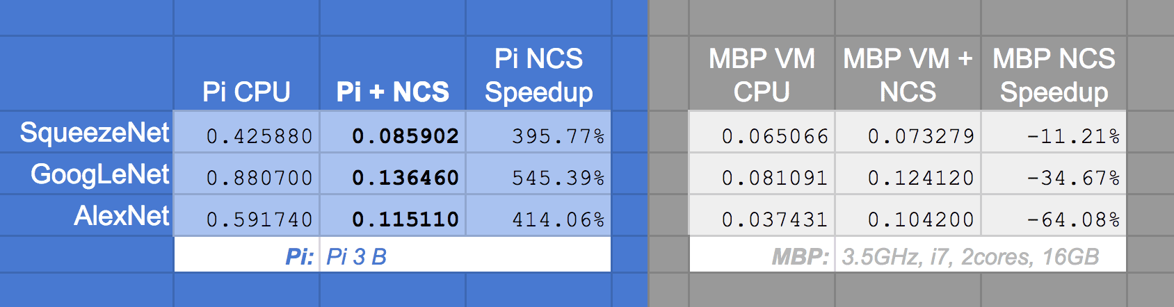
Figure 5: Intel NCS with the Raspberry Pi benchmarks. I compared classification using the Pi CPU and using the Movidius NCS. On ImageNet, the NCS achieves a 395 to 545% speedup.

The NCS is clearly faster on the Pi when compared to using the Pi’s CPU for classification achieving a 6.45x speedup (545%) on GoogLeNet. The NCS is sure to bring noticeable speed to the table on larger networks such as the three compared here.

Note: The results gathered on the Raspberry Pi used my optimized OpenCV install instructions. If you are not using the optimized OpenCV install, you would see speedups in the range of 10-11x!

When comparing execution on my MacBook Pro with Ubuntu VM to the SDK VM on my MBP, performance is worse — this is expected for a number of reasons.

For starters, my MBP has a much more powerful CPU. It turns out that it’s faster to run the full inference on the CPU versus the added overhead of moving the image from the CPU to the NCS and then pulling the results back.

Second, there is USB overhead when conducting USB passthrough to the VM. USB 3 isn’t supported via the VirtualBox USB passthrough either.

It is worth noting that the Raspberry Pi 3 B has USB 2.0. If you really want speed for a single board computer setup, select a machine that supports USB 3.0. The data transfer speeds alone will be apparent if you are benchmarking.

Next week’s results will be even more evident when we compare real-time video FPS benchmarks, so be sure to check back on Monday.

Where to from here?

I’ll be back soon with another blog post to share with you how to generate your own custom graph files for the Movidius NCS.

I’ll also be describing how to perform object detection in realtime video using the Movidius NCS — we’ll benchmark and compare the FPS speedup and I think you’ll be quite impressed.

In the meantime, be sure to check out the Movidius blog and TopCoder Competition.

Movidus blog on GitHub

Intel and Movidius are keeping their blog up to date on GitHub. Be sure to bookmark their page and/or subscribe to RSS:

developer.movidius.com/blog

You might also want to sign into GitHub and click the “watch” button on the Movidius repos:

• github.com/movidius/ncsdk
• github.com/movidius/ncappzoo

TopCoder Competition

Figure 5: Earn up to $8,000 with the Movidius NCS on TopCoder.

Are you interested in pushing the limits of the Intel Movidius Neural Compute Stick?

Intel is sponsoring a competition on TopCoder.

There are $20,000 in prizes up for grabs (first place wins $8,000)!

Registration and submission close on February 26, 2018.

Keep track of the leaderboard and standings!

Summary

Today we explored Intel’s new Movidius Neural Compute Stick. My goal here today was expose you to this new deep learning device (which we’ll  be using in future blog posts as well). I also demonstrated how to use the NCS workflow and API.

In general, the NCS workflow involes:

1. Training a network with Tensorflow or Caffe using a machine running Ubuntu/Debian (or using a pre-trained network).
2. Using the NCS SDK to generate a graph file.
3. Deploying the graph file and NCS to your single board computer running a Debian flavor of Linux. We used a Raspberry Pi 3 B running Raspbian (Debian based).
4. Performing inference, classification, object detection, etc.

Today, we skipped Steps 1 and 2. Instead I am providing graph files which you can begin using on your Pi immediately.

Then, we wrote our own classification benchmarking Python script and analyzed the results which demonstrate a significant 10x speedup on the Raspberry Pi.

I’m quite impressed with the NCS capabilities so far — it pairs quite well with the Raspberry Pi and I think it is a great value if (1) you have a use case for it or (2) you just want to hack and tinker.

I hope you enjoyed today’s introductory post on Intel’s new Movidius Neural Compute Stick!

To stay informed about PyImageSearch blog posts, sales, and events such as PyImageConf, be sure to enter your email address in the form below.

Downloads:

If you would like to download the code and images used in this post, please enter your email address in the form below. Not only will you get a .zip of the code, I’ll also send you a FREE 11-page Resource Guide on Computer Vision and Image Search Engines, including exclusive techniques that I don’t post on this blog! Sound good? If so, enter your email address and I’ll send you the code immediately!

Email address:

The post Getting started with the Intel Movidius Neural Compute Stick appeared first on PyImageSearch.

from PyImageSearch http://ift.tt/2EjpPE1
via IFTTT