Real-time object detection on the Raspberry Pi with the Movidius NCS

Today’s post is inspired by Danielle, a PyImageSearch reader who emailed me last week and asked:

Hi Adrian,

I’m enjoying your blog and I especially liked last week’s post about image classification with the Intel Movidius NCS.

I’m still considering purchasing an Intel Movidius NCS for a personal project.

My project involves object detection with the Raspberry Pi where I’m using my own custom Caffe model. The benchmark scripts you supplied for applying object detection on the Pi’s CPU were too slow and I need faster speeds.

Would the NCS be a good choice for my project and help me achieve a higher FPS?

Great question, Danielle. Thank you for asking.

The short answer is yes, you can use the Movidius NCS for object detection with your own custom Caffe model. You’ll even achieve high frame rates if you’re processing live or recorded video.

…but there’s a catch.

I told Danielle that she’ll need the full-blown Movidius SDK installed on her (Ubuntu 16.04) machine. I also mentioned that generating graph files from Caffe models isn’t always straightforward.

Inside today’s post you will learn how to:

• Install the Movidius SDK on your machine
• Generate an object detection graph file using the SDK
• Write a real-time object detection script for the Raspberry Pi + NCS

After going through the post you’ll have a good understanding of the Movidius NCS and whether it’s appropriate for your Raspberry Pi + object detection project.

To get started with real-time object detection on the Raspberry Pi, just keep reading.

Looking for the source code to this post?
Jump right to the downloads section.

Real-time object detection on the Raspberry Pi

Today’s blog post is broken into five parts.

First, we’ll install the Movidius SDK and then learn how to use the SDK to generate the Movidius graph files.

From there, we’ll write a script for real time object detection with the Intel Movidius Neural compute stick that can be used with the Pi (or alternative single board computer with minor modifications).

Next, we’ll test the script + compare results.

In a previous post, we learned how to perform real-time object detection in video on the Raspberry Pi using the CPU and the OpenCV DNN module. We achieved approximately 0.9 FPS which serves as our benchmark comparison. Today, we’re going to see how the NCS paired with a Pi performs against the Pi CPU using the same model.

And finally, I’ve captured some Frequently Asked Questions (FAQs). Refer to this section often — I expect it to grow as I receive comments and emails.

Installing the Intel Movidius SDK

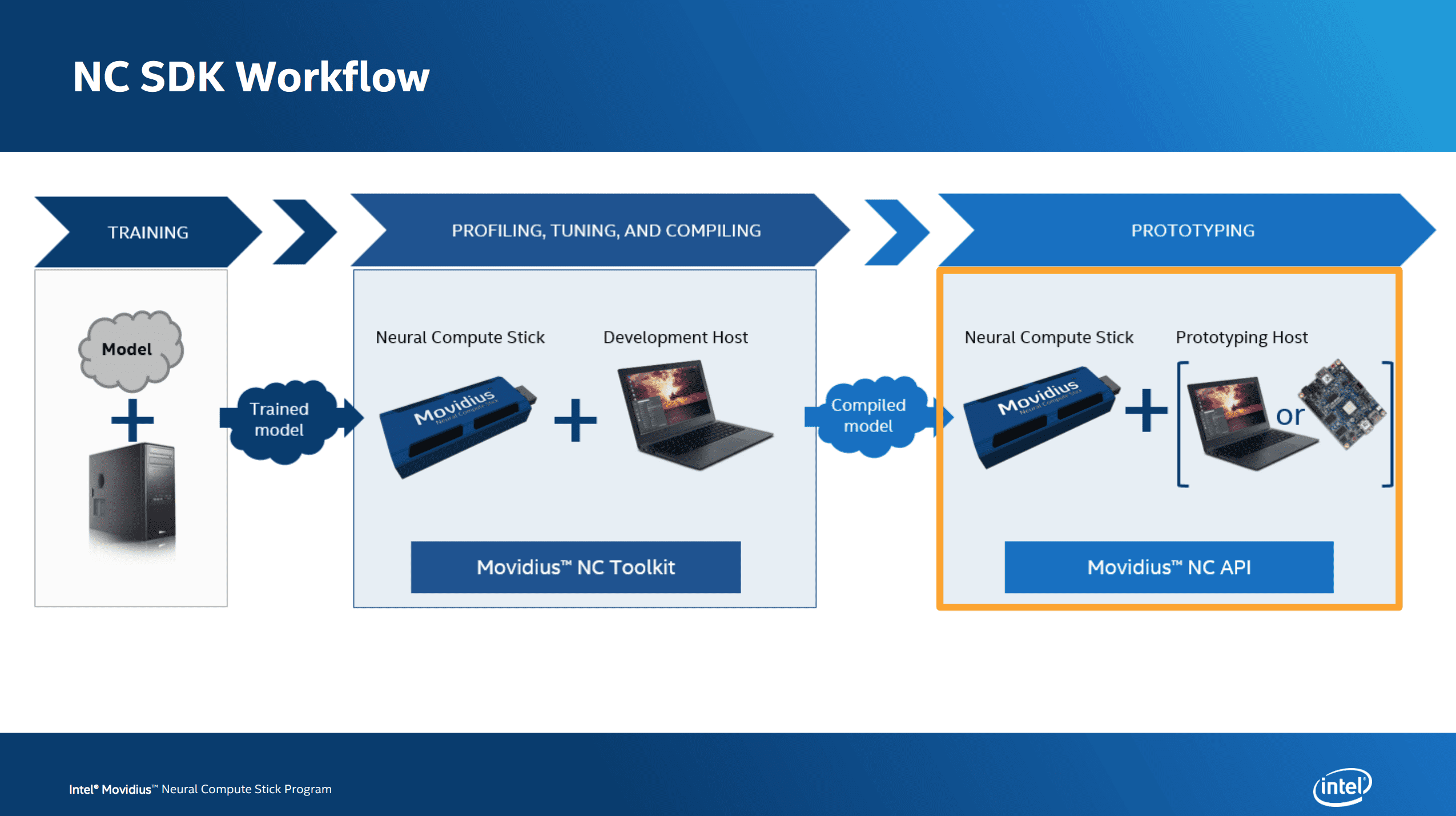
Figure 1: The Intel Movidius NCS workflow (image credit: Intel)

Last week, I reviewed the Movidius Workflow. The workflow has four basic steps:

1. Train a model using a full-size machine
2. Convert the model to a deployable graph file using the SDK and an NCS
3. Write a Python script which deploys the graph file and processes the results
4. Deploy the Python script and graph file to your single board computer equipped with an Intel Movidius NCS

In this section we’ll learn how to install the SDK which includes TensorFlow, Caffe, OpenCV, and the Intel suite of Movidius tools.

Requirements:

• Stand-alone machine or VM. We’ll install Ubuntu 16.04 LTS on it
• 30-60 minutes of time depending on download speed and machine capability
• Movidius NCS USB stick

I highlighted “Stand-alone” as it’s important that this machine only be used for Movidius development.

In other words, don’t install the SDK on a “daily development and productivity use” machine where you might have Python Virtual Environments and OpenCV installed. The install process is not entirely isolated and can/will change existing libraries on your system.

However, there is an alternative:

Use a VirtualBox Virtual Machine (or other virtualization system) and run an isolated Ubuntu 16.04 OS in the VM.

The advantage of a VM is that you can install it on your daily use machine and still keep the SDK isolated. The disadvantage is that you won’t have access to a GPU via the VM.

Danielle wants to use a Mac and VirtualBox works well on macOS, so let’s proceed down that path. Note that you could also run VirtualBox on a Windows or Linux host which may be even easier.

Before we get started, I want to bring attention to non-standard VM settings we’ll be making. We’ll be configuring USB settings which will allow the Movidius NCS to stay connected properly.

As far as I can tell from the forums, these are Mac-specific VM USB settings (but I’m not certain). Please share your experiences in the comments section.

Download Ubuntu and Virtualbox

Let’s get started.

First, download the Ubuntu 16.04 64-bit .iso image from here the official Ubuntu 16.04.3 LTS download page. You can grab the .iso directly or the torrent would also be appropriate for faster downloads.

While Ubuntu is downloading, if you don’t have Oracle VirtualBox, grab the installer that is appropriate for your OS (I’m running macOS). You can download VirtualBox here.

Non-VM users: If you aren’t going to be installing the SDK on a VM, then you can skip downloading/installing Virtualbox. Instead, scroll down to “Install the OS” but ignore the information about the VM and the virtual optical drive — you’ll probably be installing with a USB thumb drive.

After you’ve got VirtualBox downloaded, and while the Ubuntu .iso continues to download, you can install VirtualBox. Installation is incredibly easy via the wizard.

From there, since we’ll be using USB passthrough, we need the Extension Pack.

Install the Extension Pack

Let’s navigate back to the VirtualBox download page and download the Oracle VM Extension Pack if you don’t already have it.

The version of the Extension Pack must match the version of Virtualbox you are using. If you have any VMs running, you’ll want to shut them down in order to install the Extension Pack. Installing the Extension Pack is a breeze.

Create the VM

Once the Ubuntu 16.04 image is downloaded, fire up VirtualBox, and create a new VM:

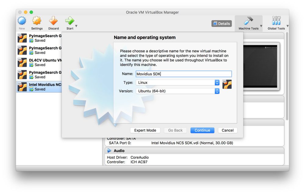
Figure 2: Creating a VM for the Intel Movidius SDK.

Give your VM reasonable settings:

• I chose 2048MB of memory for now.
• I selected 2 virtual CPUs.
• I set up a 40Gb dynamically allocated VDI (Virtualbox Disk Image).

The first two settings are easy to change later for best performance of your host and guest OSes.

As for the third setting, it is important to give your system enough space for the OS and the SDK. If you run out of space, you could always “connect” another virtual disk and mount it, or you could expand the OS disk (advanced users only).

USB passthrough settings

A VM, by definition, is virtually running as software. Inherently, this means that it does not have access to hardware unless you specifically give it permission. This includes cameras, USB, disks, etc.

This is where I had to do some digging on the intel forms to ensure that the Movidius would work with MacOS (because originally it didn’t work on my setup).

Ramana @ Intel provided “unofficial” instructions on how to set up USB over on the forums. Your mileage may vary.

In order for the VM to access the USB NCS, we need to alter settings.

Go to the “Settings” for your VM and edit “Ports > USB” to reflect a “USB 3.0 (xHCI) Controller”.

You need to set USB2 and USB3 Device Filters for the Movidius to seamlessly stay connected.

To do this, click the “Add new USB Filter” icon as is marked in this image:

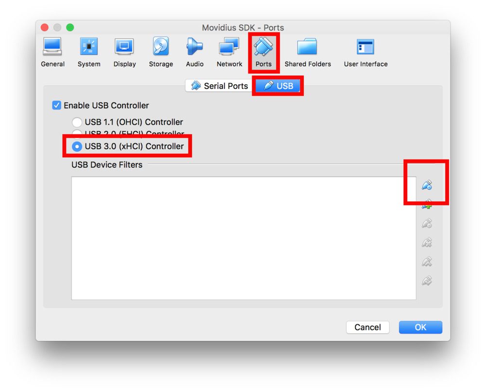
Figure 3: Adding a USB Filter in VirtualBox settings to accommodate the Intel Movidius NCS on MacOS.

From there, you need to create two USB Device Filters. Most of the fields can be left blank. I just gave each a Name and provided the Vendor ID.

1. Name: Movidius1, Vendor ID: 03e7, Other fields: blank
2. Name: Movidius2, Vendor ID: 040e, Other fields: blank

Here’s an example for the first one:

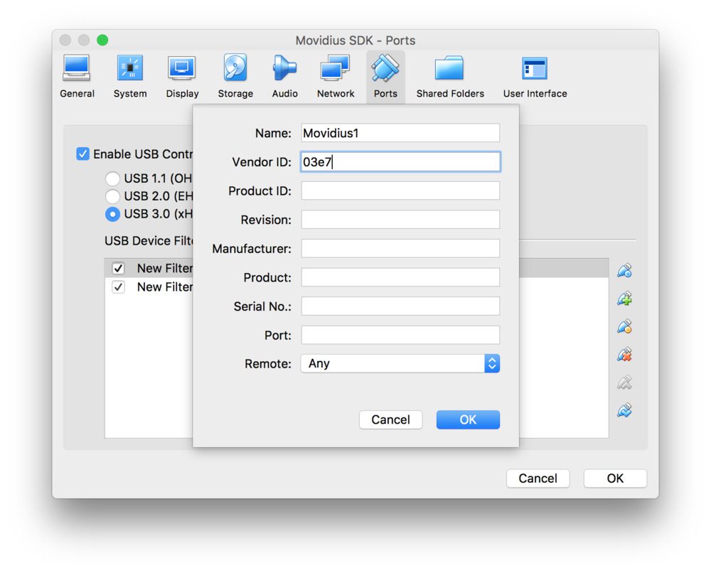
Figure 4: Two Virtualbox USB device filters are required for the Movidius NCS to work in a VM on MacOS.

Be sure to save these settings.

Install the OS

To install the OS, “insert” the .iso image into the virtual optical drive. To do this, go to “Settings”, then under “Storage” select “Controller: IDE > Empty”, and click the disk icon (marked by the red box).  Then find and select your freshly downloaded Ubuntu .iso.

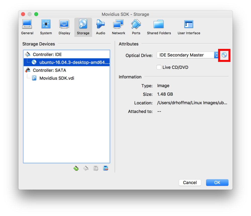
Figure 5: Inserting an Ubuntu 16.04 .iso file into a Virtualbox VM.

Verify all settings and then boot your machine.

Follow the prompts to “Install Ubuntu”. If you have a fast internet connection, you can select “Download updates while installing Ubuntu”.  I did not select the option to “Install third-party software…”.

The next step is to “Erase disk and install Ubuntu” — this is a safe action because we just created the empty VDI disk. From there, set up system name and a username + password.

Once you’ve been instructed to reboot and removed the virtual optical disk, you’re nearly ready to go.

First, let’s update our system. Open a terminal and type the following to update your system:

$ sudo apt-get update && sudo apt-get upgrade

Install Guest Additions

Non-VM users: You should skip this section.

From there, since we’re going to be using a USB device (the Intel NCS), let’s install guest additions. Guest additions also allows for bidirectional copy/paste between the VM and the host amongst other nice sharing utilities.

Guest additions can be installed by going to the Devices menu of Virtual box and clicking “Insert Guest Additions CD Image…”:

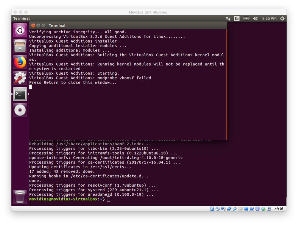
Figure 6: Virtualbox Guest Additions for Ubuntu has successfully been installed.

Follow the prompt to press “Return to close this window…” which completes the the install.

Take a snapshot

Non-VM users: You can skip this section or make a backup of your system via your preferred method.

From there, I like to reboot followed by taking a “snapshot” of my VM.

Rebooting is important because we just updated and installed a lot of software and want to ensure the changes take effect.

Additionally, a snapshot will allow us to rollback if we make any mistakes or have problems during the install — as we’ll find out, there are some gotchas along the way that can trip you up wih the Movidius SDK, so this is a worthwhile step.

Definitely take the time to snapshot your system. Go to the VirtualBox menubar and press “Machine > Take Snapshot”.

You can give the snapshot a name such as “Installed OS and Guest Additions” as is shown below:

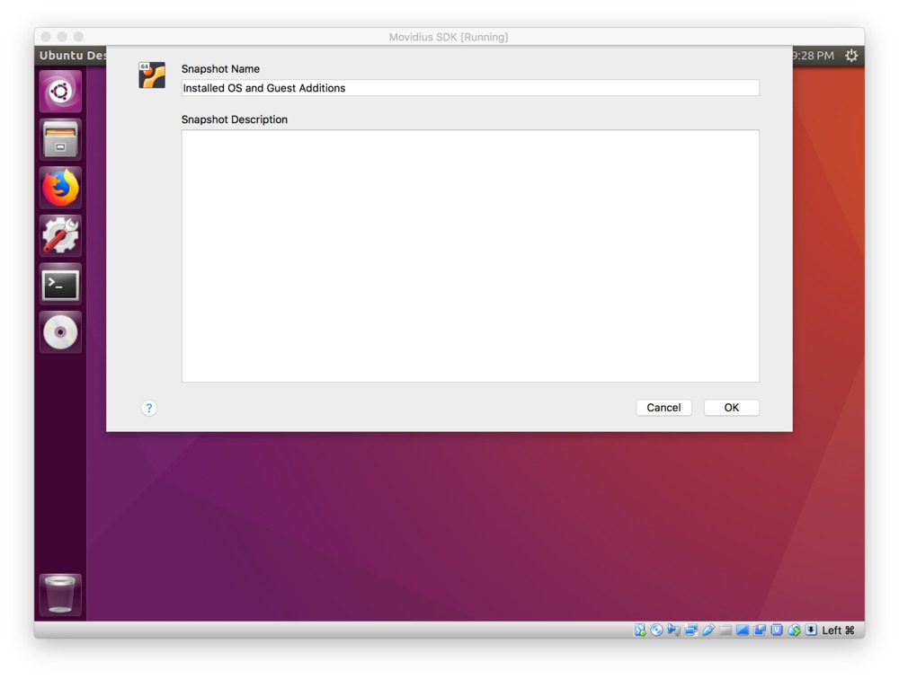
Figure 7: Taking a snapshot of the Movidius SDK VM prior to actually installing the SDK.

Installing the Intel Movidius SDK on Ubuntu

This section assumes that you either (a) followed the instructions above to install Ubuntu 16.04 LTS on a VM, or (b) are working with a fresh install of Ubuntu 16.04 LTS on a Desktop/Laptop.

Intel makes the process of installing the SDK very easy. Cheers to that!

But like I said above, I wish there was an advanced method. I like easy, but I also like to be in control of my computer.

Let’s install Git from a terminal:

$ sudo apt-get install git

From there, let’s follow Intel’s instructions very closely so that there are hopefully no issues.

Open a terminal and follow along:

$ cd ~
$ mkdir workspace
$ cd workspace

Now that we’re in the workspace, let’s clone down the NCSDK and the NC App Zoo:

$ git clone https://github.com/movidius/ncsdk.git
$ git clone https://github.com/movidius/ncappzoo.git

And from there, you should navigate into the

ncsdk

  directory and install the SDK:

$ cd ~/workspace/ncsdk
$ make install

You might want to go outside for some fresh air or grab yourself a cup of coffee (or beer depending on what time it is). This process will take about 15 minutes depending on the capability of your host machine and your download speed.

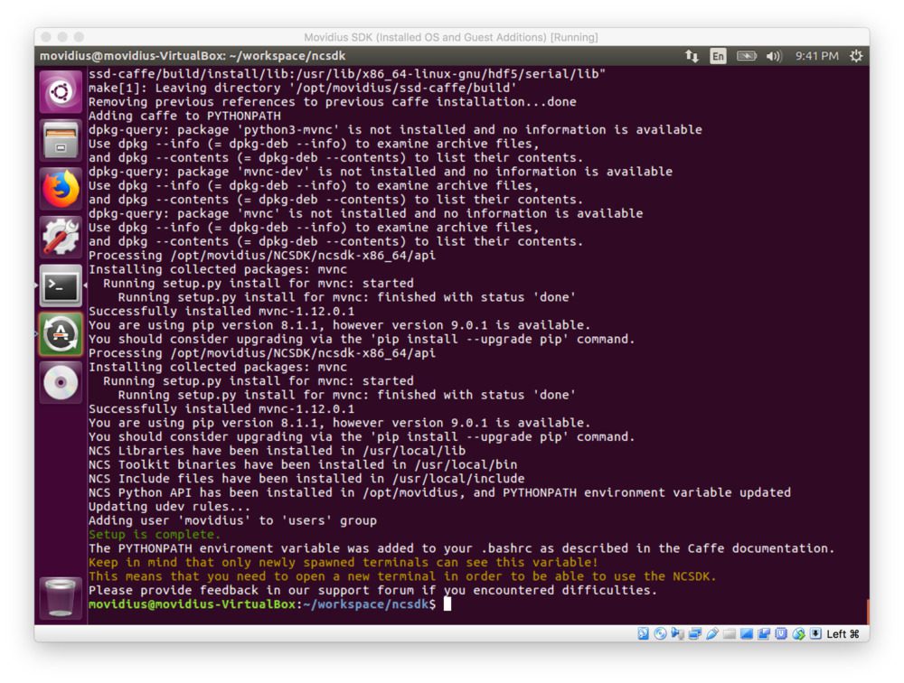
Figure 8: The Movidius SDK has been successfully installed on our Ubuntu 16.04 VM.

VM Users: Now that the installation is complete, it would be a good time to take another snapshot so we can revert in the future if needed. You can follow the same method as above to take another snapshot (I named mine “SDK installed”). Just remember that snapshots require adequate disk space on the host.

Connect the NCS to a USB port and verify connectivity

Non-VM users: You can skip this step because you’ll likely not have any USB issues. Instead, plug in the NCS and scroll to “Test the SDK”.

First, connect your NCS to the physical USB port on your laptop or desktop.

Note: Given that my Mac has Thunderbolt 3 / USB-C ports, I initially plugged in Apple’s USB-C Digital AV Multiport Adapter which has a USB-A and HDMI port. This didn’t work. Instead, I elected to use a simple adapter, but not a USB hub. Basically you should try to eliminate the need for any additional required drivers if you’re working with a VM.

From there, we need to make the USB stick accessible to the VM. Since we have Guest Additions and the Extension Pack installed, we can do this from the VirtualBox menu. In the VM menubar, click “Devices > USB > ‘Movidius Ltd. Movidius MA2X5X'” (or a device with a similar name). It’s possible that the Movidus already has a checkmark next to it, indicating that it is connected to the VM.

In the VM open a terminal. You can run the following command to verify that the OS knows about the USB device:

$ dmesg

You should see that the Movidius is recognized by reading the most recent 3 or 4 log messages as shown below:

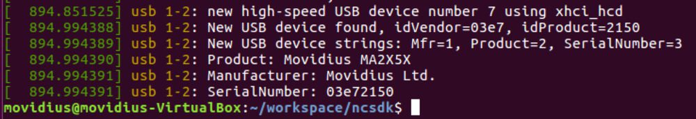
Figure 9: Running the dmesg command in a terminal allows us to see that the Movidius NCS is associated with the OS.

If you see the Movidius device then it’s time to test the installation.

Test the SDK

Now that the SDK is installed, you can test the installation by running the pre-built examples:

$ cd ~/workspace/ncsdk
$ make examples

This may take about five minutes to run and you’ll see a lot of output (not shown in the block above).

If you don’t see error messages while all the examples are running, that is good news. You’ll notice that the Makefile has executed code to go out and download models and weights from Github, and from there it runs mvNCCompile. We’ll learn about mvNCCompile in the next section. I’m impressed with the effort put into the Makefiles by the Movidius team.

Another check (this is the same one we did on the Pi last week):

$ cd ~/workspace/ncsdk/examples/apps
$ make all
$ cd hello_ncs_py
$ python hello_ncs.py
Hello NCS! Device opened normally.
Goodbye NCS! Device closed normally.
NCS device working.

This test ensures that the links to your API and connectivity to the NCS are working properly.

If you’ve made it this far without too much trouble, then congratulations!

Generating Movidius graph files from your own Caffe models

Generating graph files is made quite easy by Intel’s SDK. In some cases you can actually compute the graph using a Pi. Other times, you’ll need a machine with more memory to accomplish the task.

There’s one main tool that I’d like to share with you:

mvNCCompile

 .

This command line tool supports both TensorFlow and Caffe. It is my hope that Keras will be supported in the future by Intel.

For Caffe, the command line arguments are in the following format (TensorFlow users should refer to the documentation which is similar):

$ mvNCCompile network.prototxt -w network.caffemodel \
        -s MaxNumberOfShaves -in InputNodeName -on OutputNodeName \
        -is InputWidth InputHeight -o OutputGraphFilename

Let’s review the arguments:

• network.prototxt
  

   : path/filename of the network file

• -w network.caffemodel
  

   : path/filename of the caffemodel file

• -s MaxNumberOfShaves
  

   : SHAVEs (1, 2, 4, 8, or 12) to use for network layers (I think the default is 12, but the documentation is unclear)

• -in InputNodeNodeName
  

   : you may optionally specify a specific input layer (it would match the name in the prototxt file)

• -on OutputNodeName
  

   : by default the network is processed through the output tensor and this option allows a user to select an alternative end point in the network

• -is InputWidth InputHeight
  

   : the input shape is very important and should match the design of your network

• -o OutputGraphFilename
  

   : if no file/path is specified this defaults to the very ambiguous filename,

  graph
  

   , in the current working directory

Where’s the batch size argument?

The batch size for the NCS is always 1 and the number of color channels is assumed to be 3.

If you provide command line arguments to

mvNCCompile

  in the right format with an NCS plugged in, then you’ll be on your way to having a graph file rather quickly.

There’s one caveat (at least from my experience thus far with Caffe files). The

mvNCCompile

  tool requires that the prototxt be in a specific format.

You might have to modify your prototxt to get the

mvNCCompile

  tool to work. If you’re having trouble, the Movidius forums may be able to guide you.

Today we’re working with MobileNet Single Shot Detector (SSD) trained with Caffe. The GitHub user, chuanqui305, gets credit for the training the model on the MS-COCO dataset. Thank you chuanqui305!

I have provided chuanqui305’s files in the “Downloads” section. To compile the graph you should execute the following command:

$ mvNCCompile models/MobileNetSSD_deploy.prototxt \
        -w models/MobileNetSSD_deploy.caffemodel \
        -s 12 -is 300 300 -o graphs/mobilenetgraph
mvNCCompile v02.00, Copyright @ Movidius Ltd 2016

/usr/local/bin/ncsdk/Controllers/FileIO.py:52: UserWarning: You are using a large type. Consider reducing your data sizes for best performance
  "Consider reducing your data sizes for best performance\033[0m")

You should expect the Copyright message and possibly additional information or a warning like I encountered above. I procdeded by ignoring the warning without any trouble.

Object detection with the Intel Movidius Neural Compute Stick

Let’s write a real-time object detection script. The script very closely aligns with the non-NCS version that we built in a previous post.

You can find today’s script and associated files in the “Downloads” section of this blog post. I suggest you download the source code and model file if you wish to follow along.

Once you’ve downloaded the files, open

ncs_realtime_objectdetection.py

 :

# import the necessary packages
from mvnc import mvncapi as mvnc
from imutils.video import VideoStream
from imutils.video import FPS
import argparse
import numpy as np
import time
import cv2

We import our packages on Lines 2-8, taking note of the

mvncapi

, which is the the Movidius NCS Python API package.

From there we’ll perform initializations:

# initialize the list of class labels our network was trained to
# detect, then generate a set of bounding box colors for each class
CLASSES = ["background", "aeroplane", "bicycle", "bird",
        "boat", "bottle", "bus", "car", "cat", "chair", "cow",
        "diningtable", "dog", "horse", "motorbike", "person",
        "pottedplant", "sheep", "sofa", "train", "tvmonitor"]
COLORS = np.random.uniform(0, 255, size=(len(CLASSES), 3))

# frame dimensions should be sqaure
PREPROCESS_DIMS = (300, 300)
DISPLAY_DIMS = (900, 900)

# calculate the multiplier needed to scale the bounding boxes
DISPLAY_MULTIPLIER = DISPLAY_DIMS[0] // PREPROCESS_DIMS[0]

Our class labels and associated random colors (one random color per class label) are initialized on Lines 12-16.

Our MobileNet SSD requires dimensions of 300×300, but we’ll be displaying the video stream at 900×900 to better visualize the output (Lines 19 and 20).

Since we’re changing the dimensions of the image, we need to calculate the scalar value to scale our object detection boxes (Line 23).

From there we’ll define a

preprocess_image

  function:

def preprocess_image(input_image):
        # preprocess the image
        preprocessed = cv2.resize(input_image, PREPROCESS_DIMS)
        preprocessed = preprocessed - 127.5
        preprocessed = preprocessed * 0.007843
        preprocessed = preprocessed.astype(np.float16)

        # return the image to the calling function
        return preprocessed

The actions made in this pre-process function are specific to our MobileNet SSD model. We resize, perform mean subtraction, scale the image, and convert it to

float16

  format (Lines 27-30).

Then we return the

preprocessed

  image to the calling function (Line 33).

To learn more about pre-processing for deep learning, be sure to refer to my book, Deep Learning for Computer Vision with Python.

From there we’ll define a

predict

  function:

def predict(image, graph):
        # preprocess the image
        image = preprocess_image(image)

        # send the image to the NCS and run a forward pass to grab the
        # network predictions
        graph.LoadTensor(image, None)
        (output, _) = graph.GetResult()

        # grab the number of valid object predictions from the output,
        # then initialize the list of predictions
        num_valid_boxes = output[0]
        predictions = []

This

predict

  function applies to users of the Movidius NCS and it is largely based on the Movidius NC App Zoo GitHub example — I made a few minor modifications.

The function requires an

image

  and a

graph

  object (which we’ll instantiate later).

First we pre-process the image (Line 37).

From there, we run a forward pass through the neural network utilizing the NCS while grabbing the predictions (Lines 41 and 42).

Then we extract the number of valid object predictions (

num_valid_boxes

 ) and initialize our

predictions

  list (Lines 46 and 47).

From there, let’s loop over the valid results:

# loop over results
        for box_index in range(num_valid_boxes):
                # calculate the base index into our array so we can extract
                # bounding box information
                base_index = 7 + box_index * 7

                # boxes with non-finite (inf, nan, etc) numbers must be ignored
                if (not np.isfinite(output[base_index]) or
                        not np.isfinite(output[base_index + 1]) or
                        not np.isfinite(output[base_index + 2]) or
                        not np.isfinite(output[base_index + 3]) or
                        not np.isfinite(output[base_index + 4]) or
                        not np.isfinite(output[base_index + 5]) or
                        not np.isfinite(output[base_index + 6])):
                        continue

                # extract the image width and height and clip the boxes to the
                # image size in case network returns boxes outside of the image
                # boundaries
                (h, w) = image.shape[:2]
                x1 = max(0, int(output[base_index + 3] * w))
                y1 = max(0, int(output[base_index + 4] * h))
                x2 = min(w,     int(output[base_index + 5] * w))
                y2 = min(h,     int(output[base_index + 6] * h))

                # grab the prediction class label, confidence (i.e., probability),
                # and bounding box (x, y)-coordinates
                pred_class = int(output[base_index + 1])
                pred_conf = output[base_index + 2]
                pred_boxpts = ((x1, y1), (x2, y2))

                # create prediciton tuple and append the prediction to the
                # predictions list
                prediction = (pred_class, pred_conf, pred_boxpts)
                predictions.append(prediction)

        # return the list of predictions to the calling function
        return predictions

Okay, so the above code might look pretty ugly. Let’s take a step back. The goal of this loop is to append prediction data to our

predictions

  list in an organized fashion so we can use it later. This loop just extracts and organizes the data for us.

But what in the world is the

base_index

 ?

Basically, all of our data is stored in one long array/list (

output

 ). Using the

box_index

 , we calculate our

base_index

  which we’ll then use (with more offsets) to extract prediction data.

I’m guessing that whoever wrote the Python API/bindings is a C/C++ programmer. I might have opted for a different way to organize the data such as a list of tuples like we’re about to construct.

Why are we ensuring values are finite on Lines 55-62?

This ensures that we have valid data. If it’s invalid we

continue

  back to the top of the loop (Line 63) and try another prediction.

What is the format of the

output

  list?

The output list has the following format:

0. output[0]
   

    : we extracted this value on Line 46 as

   num_valid_boxes
   

1. output[base_index + 1]
   

    : prediction class index

2. output[base_index + 2]
   

    : prediction confidence

3. output[base_index + 3]
   

    : object boxpoint x1 value (it needs to be scaled)

4. output[base_index + 4]
   

    : object boxpoint y1 value (it needs to be scaled)

5. output[base_index + 5]
   

    : object boxpoint x2 value (it needs to be scaled)

6. output[base_index + 6]
   

    : object boxpoint y2 value (it needs to be scaled)

Lines 68-82 handle building up a single prediction tuple. The prediction consists of:

(pred_class, pred_conf, pred_boxpts)

  and we append the

prediction

  to the

predictions

  list on Line 83.

After we’re done looping through the data, we

return

  the

predictions

  list to the calling function on Line 86.

From there, let’s parse our command line arguments:

# construct the argument parser and parse the arguments
ap = argparse.ArgumentParser()
ap.add_argument("-g", "--graph", required=True,
        help="path to input graph file")
ap.add_argument("-c", "--confidence", default=.5,
        help="confidence threshold")
ap.add_argument("-d", "--display", type=int, default=0,
        help="switch to display image on screen")
args = vars(ap.parse_args())

We parse our three command line arguments on Lines 89-96.

We require the path to our graph file. Optionally we can specify a different confidence threshold or display the image to the screen.

Next, we’ll connect to the NCS and load the graph file onto it:

# grab a list of all NCS devices plugged in to USB
print("[INFO] finding NCS devices...")
devices = mvnc.EnumerateDevices()

# if no devices found, exit the script
if len(devices) == 0:
        print("[INFO] No devices found. Please plug in a NCS")
        quit()

# use the first device since this is a simple test script
# (you'll want to modify this is using multiple NCS devices)
print("[INFO] found {} devices. device0 will be used. "
        "opening device0...".format(len(devices)))
device = mvnc.Device(devices[0])
device.OpenDevice()

# open the CNN graph file
print("[INFO] loading the graph file into RPi memory...")
with open(args["graph"], mode="rb") as f:
        graph_in_memory = f.read()

# load the graph into the NCS
print("[INFO] allocating the graph on the NCS...")
graph = device.AllocateGraph(graph_in_memory)

The above block is identical to last week, so I’m not going to review it in detail. Essentially we’re checking that we have an available NCS, connecting, and loading the graph file on it.

The result is a

graph

  object which we use in the predict function above.

Let’s kick off our video stream:

# open a pointer to the video stream thread and allow the buffer to
# start to fill, then start the FPS counter
print("[INFO] starting the video stream and FPS counter...")
vs = VideoStream(usePiCamera=True).start()
time.sleep(1)
fps = FPS().start()

We start the camera

VideoStream

 , allow our camera to warm up, and our instantiate our FPS counter.

Now let’s process the camera feed frame by frame:

# loop over frames from the video file stream
while True:
        try:
                # grab the frame from the threaded video stream
                # make a copy of the frame and resize it for display/video purposes
                frame = vs.read()
                image_for_result = frame.copy()
                image_for_result = cv2.resize(image_for_result, DISPLAY_DIMS)

                # use the NCS to acquire predictions
                predictions = predict(frame, graph)

Here we’re reading a frame from the video stream, making a copy (so we can draw on it later), and resizing it (Lines 135-137).

We then send the frame through our object detector which will return

predictions

  to us.

Let’s loop over the

predictions

  next:

# loop over our predictions
                for (i, pred) in enumerate(predictions):
                        # extract prediction data for readability
                        (pred_class, pred_conf, pred_boxpts) = pred

                        # filter out weak detections by ensuring the `confidence`
                        # is greater than the minimum confidence
                        if pred_conf > args["confidence"]:
                                # print prediction to terminal
                                print("[INFO] Prediction #{}: class={}, confidence={}, "
                                        "boxpoints={}".format(i, CLASSES[pred_class], pred_conf,
                                        pred_boxpts))

Looping over the

predictions

 , we first extract the class, confidence and boxpoints for the object (Line 145).

If the

confidence

  is above the threshold, we print the prediction to the terminal and check if we should display the image on the screen:

# check if we should show the prediction data
                                # on the frame
                                if args["display"] > 0:
                                        # build a label consisting of the predicted class and
                                        # associated probability
                                        label = "{}: {:.2f}%".format(CLASSES[pred_class],
                                                pred_conf * 100)

                                        # extract information from the prediction boxpoints
                                        (ptA, ptB) = (pred_boxpts[0], pred_boxpts[1])
                                        ptA = (ptA[0] * DISP_MULTIPLIER, ptA[1] * DISP_MULTIPLIER)
                                        ptB = (ptB[0] * DISP_MULTIPLIER, ptB[1] * DISP_MULTIPLIER)
                                        (startX, startY) = (ptA[0], ptA[1])
                                        y = startY - 15 if startY - 15 > 15 else startY + 15

                                        # display the rectangle and label text
                                        cv2.rectangle(image_for_result, ptA, ptB,
                                                COLORS[pred_class], 2)
                                        cv2.putText(image_for_result, label, (startX, y),
                                                cv2.FONT_HERSHEY_SIMPLEX, 1, COLORS[pred_class], 3)

If we’re displaying the image, we first build a

label

  string which will contain the class name and confidence in percentage form (Lines 160-161).

From there we extract the corners of the rectangle and calculate the position for our

label

  relative to those points (Lines 164-168).

Finally, we display the rectangle and text label on the screen. If there are multiple objects of the same class in the frame, the boxes and labels will have the same color.

From there, let’s display the image and update our FPS counter:

# check if we should display the frame on the screen
                # with prediction data (you can achieve faster FPS if you
                # do not output to the screen)
                if args["display"] > 0:
                        # display the frame to the screen
                        cv2.imshow("Output", image_for_result)
                        key = cv2.waitKey(1) & 0xFF

                        # if the `q` key was pressed, break from the loop
                        if key == ord("q"):
                                break

                # update the FPS counter
                fps.update()
        
        # if "ctrl+c" is pressed in the terminal, break from the loop
        except KeyboardInterrupt:
                break

        # if there's a problem reading a frame, break gracefully
        except AttributeError:
                break

Outside of the prediction loop, we again make a check to see if we should display the frame to the screen. If so, we show the frame (Line 181) and wait for the “q” key to be pressed if the user wants to quit (Lines 182-186).

We update our frames per second counter on Line 189.

From there, we’ll most likely continue to the top of the frame-by-frame loop to complete the process again.

If the user happened to press “ctrl+c” in the terminal or if there’s a problem reading a frame, we break out of the loop.

# stop the FPS counter timer
fps.stop()

# destroy all windows if we are displaying them
if args["display"] > 0:
        cv2.destroyAllWindows()

# stop the video stream
vs.stop()

# clean up the graph and device
graph.DeallocateGraph()
device.CloseDevice()

# display FPS information
print("[INFO] elapsed time: {:.2f}".format(fps.elapsed()))
print("[INFO] approx. FPS: {:.2f}".format(fps.fps()))

This last code block handles some housekeeping (Lines 200-211) and finally prints the elapsed time and the frames per second pipeline information to the screen. This information allows us to benchmark our script.

Movidius NCS object detection results

Let’s run our real-time object detector with the NCS using the following command:

$ python ncs_realtime_objectdetection.py --graph graph --display 1

Prediction results will be printed in the terminal and the image will be displayed on our Raspberry Pi monitor.

Below I have included an example GIF animation of shooting a video with a smartphone and then post-processing it on the Raspberry Pi:

Thank you to David McDuffee for shooting these example clips so I could include it!

Here’s an example video of the system in action recorded with a Raspberry Pi:

A big thank you to David Hoffman for demoing the Raspberry Pi + NCS in action.

Note: As some of you know, this past week I was taking care of a family member who is recovering from emergency surgery. While I was able to get the blog post together, I wasn’t able to shoot the example videos. A big thanks to both David Hoffman and David McDuffee for gathering great examples making today’s post possible!

And here’s a table of results:

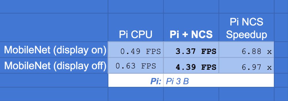
Figure 10: Object detection results on the Intel Movidius Neural Comput Stick (NCS) when compared to the Pi CPU. The NCS helps the Raspberry Pi to achieve a ~6.88x speedup.

The Movidius NCS can propel the Pi to a ~6.88x speedup over the standard CPU object detection! That’s progress.

I reported results with the display option being “on” as well as “off”. As you can see, displaying on the screen slows down the FPS by about 1 FPS due to the OpenCV drawing text/boxes as well as highgui overhead. The reason I reported both this week is so that you’ll have a better idea of what to expect if you’re using this platform and performing object detection without the need for a display (such as in a robotics application).

Note: Optimized OpenCV 3.3+ (with the DNN module) installations will have faster FPS on the Pi CPU (I reported 0.9 FPS previously). To install OpenCV with NEON and VFP3 optimizations just read this previous post. I’m not sure if the version of OpenCV 2.4 that gets installed with the Movidius toolchain contains these optimizations which is one reason why I reported the non-optimized 0.49 FPS metric in the table.

I’ll wrap up this section by saying that it is possible give the illusion of faster FPS with threading if you so wish. Check out this previous post and implement the strategy into

ncs_realtime_objectdetection.py

  that we reviewed today.

Frequently asked questions (FAQs)

In this section I detail the answers to Frequently Asked Questions regarding the NCS.

Why does my Movidius NCS continually disconnect from my VM? It appears to be connected, but then when I run ‘make examples’ as instructed above, I see connectivity error messages. I’m running macOS and using a VM.

You must use the VirtualBox Extension Pack and add two USB device filters specifically for the Movidius. Please refer to the USB passthrough settings above.

No predictions are being made on the video — I can see the video on the screen, but I don’t see any error messages or stacktrace. What might be going wrong?

This is likely due to an error in pre-processing.

Be sure your pre-processing function is correctly performing resizing and normalization.

First, the dimensions of the pre-processed image must match the model exactly. For the MobileNet SSD that I’m working with, it is 300×300.

Second, you must normalize the input via mean subtraction and scaling.

I just bought an NCS and want to run the example on my Pi using my HDMI monitor and a keyboard/mouse. How do I access the USB ports that the NCS is blocking?

It seems a bit of poor design that the NCS blocks adjacent USB ports. The only solution I know of is to buy a short extension cable such as this 6in USB 3.0 compatible cable on Amazon — this will give more space around the other three USB ports.

Of course, you could also take your NCS to a machine shop and mill down the heatsink, but that wouldn’t be good for your warranty or cooling purposes.

How do I install the Python bindings to the NCS SDK API in a virtual environment?

Quite simply: you can’t.

Install the SDK on an isolated computer or VM.

For your Pi, install the SDK API-only mode on a separate micro SD card than the one you currently use for everyday use.

I have errors when running ‘mvNCCompile’ on my models. What do you recommend?

The Movidius graph compiling tool, mvNCCompile, is very particular about the input files. Oftentimes for Caffe, you’ll need to modify the .prototxt file. For TensorFlow I’ve seen that the filenames themselves need to be in a particular format.

Generally it is a simple change that needs to be made, but I don’t want to lead you in the wrong direction. The best resource right now is the Movidius Forums.

In the future, I may update these FAQs and the Generating Movidius graph files from your own Caffe models section with guidelines or a link to Intel documentation.

I’m hoping that the Movidius team at Intel can improve their graph compiler tool as well.

What’s next?

If you’re looking to perform image classification with your NCS, then refer to last week’s blog post.

Let me know what you’re looking to accomplish with a Movidius NCS and maybe I’ll turn the idea into a blog post.

Be sure to check out the Movidius blog and TopCoder Competition as well.

Movidus blog on GitHub

The Movidius team at Intel has a blog where you’ll find additional information:

developer.movidius.com/blog

The GitHub community surrounding the Movidius NCS is growing. I recommend that you search for Movidius projects using the GitHub search feature.

Two official repos that you should watch are (click the “watch” button on to be informed of updates):

• github.com/movidius/ncsdk
• github.com/movidius/ncappzoo

TopCoder Competition

Figure 11: Earn up to $8,000 with the Movidius NCS on TopCoder.

Are you interested earning up to $8,000?

Intel is sponsoring a competition on TopCoder.

There are $20,000 in prizes up for grabs (first place wins $8,000)!

Registration and submission closes on February 26, 2018. That is next Monday, so don’t waste any time!

Keep track of the leaderboard and standings!

Summary

Today, we answered PyImageSearch reader, Danielle’s questions. We learned how to:

• Install the SDK in a VM so she can use her Mac.
• Generate Movidius graph files from Caffe models.
• Perform object detection with the Raspberry Pi and NCS.

We saw that MobileNet SSD is >6.8x faster on a Raspberry Pi when using the NCS.

The Movidius NCS is capable of running many state-of-the-art networks and is a great value at less than $100 USD. You should consider purchasing one if you want to deploy it in a project or if you’re just yearning for another device to tinker with. I’m loving mine.

There is a learning curve, but the Movidius team at Intel has done a decent job breaking down the barrier to entry with working Makefiles on GitHub.

There is of course room for improvement, but nobody said deep learning was easy.

I’ll wrap today’s post by asking a simple question:

Are you interested in learning the fundamentals of deep learning, how to train state-of-the-art networks from scratch, and discovering my handpicked best practices?

If that sounds good, then you should definitely check out my latest book, Deep Learning for Computer Vision with Python. It is jam-packed with practical information and deep learning code that you can use in your own projects.

Downloads:

If you would like to download the code and images used in this post, please enter your email address in the form below. Not only will you get a .zip of the code, I’ll also send you a FREE 11-page Resource Guide on Computer Vision and Image Search Engines, including exclusive techniques that I don’t post on this blog! Sound good? If so, enter your email address and I’ll send you the code immediately!

Email address:

The post Real-time object detection on the Raspberry Pi with the Movidius NCS appeared first on PyImageSearch.

from PyImageSearch http://ift.tt/2HuPhIH
via IFTTT