Today’s blog post is on image hashing — and it’s the hardest blog post I’ve ever had to write.
Image hashing isn’t a particularly hard technique (in fact, it’s one of the easiest algorithms I’ve taught here on the PyImageSearch blog).
But the subject matter and underlying reason of why I’m covering image hashing today of all days nearly tear my heart out to discuss.
The remaining introduction to this blog post is very personal and covers events that happened in my life five years ago, nearly to this very day.
If you want to skip the personal discussion and jump immediately to the image hashing content, I won’t judge — the point of PyImageSearch is to be a computer vision blog after all.
To skip to the computer vision content, just scroll to the “Image Hashing with OpenCV and Python” section where I dive into the algorithm and implementation.
But while PyImageSearch is a computer vision and deep learning blog, I am a very real human that writes it.
And sometimes the humanity inside me needs a place to share.
A place to share about childhood.
Mental illness.
And the feelings of love and loss.
I appreciate you as a PyImageSearch reader and I hope you’ll let me have this introduction to write, pour out, and continue my journey to finding peace.
My best friend died in my arms five years ago, nearly to this very day.
Her name was Josie.
Some of you may recognize this name — it appears in the dedication of all my books and publications.
Josie was a dog, a perfect, loving, caring beagle, that my dad got for me when I was 11 years old.
Perhaps you already understand what it’s like to lose a childhood pet.
Or perhaps you don’t see the big deal — “It’s only a dog, right?”
But to me, Josie was more than a dog.
She was the last thread that tied my childhood to my adulthood. Any unadulterated feelings of childhood innocence were tied to that thread.
When that thread broke, I nearly broke too.
You see, my childhood was a bit of a mess, to say the least.
I grew up in a broken home. My mother suffered (and still does) from bipolar schizophrenia, depression, severe anxiety, and a host of other mental afflictions, too many for me to enumerate.
Without going into too much detail, my mother’s illnesses are certainly not her fault — but she often resisted the care and help she so desperately needed. And when she did accept help, if often did not go well.
My childhood consisted of a (seemingly endless) parade of visitations to the psychiatric hospital followed by nearly catatonic interactions with my mother. When she came out of the catatonia, my home life often descended into turmoil and havoc.
You grow up fast in that environment.
And it becomes all too easy to lose your childhood innocence.
My dad, who must have recognized the potentially disastrous trajectory my early years were on (and how it could have a major impact on my well-being as an adult), brought home a beagle puppy for me when I was 11 years old, most likely to help me hold on to a piece of my childhood.
He was right. And it worked.
As a kid, there is no better feeling than holding a puppy, feeling its heartbeat against yours, playfully squirming and wiggling in and out of your arms, only to fall asleep on your lap five minutes later.
Josie gave me back some of my child innocence.
Whenever I got home from school, she was there.
Whenever I sat by myself, playing video games late at night (a ritual I often performed to help me “escape” and cope), she was there.
And whenever my home life turned into screaming, yelling, and utterly incomprehensible shrieks of tortured mental illness, Josie was always right there next to me.
As I grew into those awkward mid-to-late teenage years, I started to suffer from anxiety issues myself, a condition, I later learned, all too common for kids growing up in these circumstances.
During freshman and sophomore year of high school my dad had to pick me up and take me home from the school nurse’s office no less than twenty times due to me having what I can only figure were acute anxiety attacks.
Despite my own issues as a teenager, trying to grow up and somehow grasp what was going on with myself and my family, Josie always laid next to me, keeping me company, and reminding me of what it was like to be a kid.
But when Josie died in my arms five years ago that thread broke — that single thread was all that tied the “adult me” to the “childhood me”.
The following year was brutal. I was finishing up my final semester of classes for my PhD, about to start my dissertation. I was working full-time. And I even had some side projects going on…
…all the while trying to cope with not only the loss of my best friend, but also the loss of my childhood as well.
It was not a good year and I struggled immensely.
However, soon after Josie died I found a bit of solace in collecting and organizing all the photos my family had of her.
This therapeutic, nostalgic task involved scanning physical photos, going through old SD cards for digital cameras, and even digging through packed away boxes to find long forgotten cellphones that had pictures on their memory cards.
When I wasn’t working or at school I spent a lot of time importing all these photos into iPhoto on my Mac. It was tedious, manual work but that was just the work I needed.
However, by the time I got ~80% of the way done importing the photos the weight became too much for me to bear on my shoulders. I needed to take a break for my own mental well-being.
It’s now been five years.
I still have that remaining 20% to finish — and that’s exactly what I’m doing now.
I’m in a much better place now, personally, mentally, and physically. It’s time for me to finish what I started, if for no other reason than than I owe it to myself and to Josie.
The problem is that it’s been five years since I’ve looked at these directories of JPEGs.
Some directories have been imported into iPhoto (where I normally look at photos).
And others have not.
I have no idea which photos are already in iPhoto.
So how am I going to go about determining which directories of photos I still need to sort through and then import/organize?
The answer is image hashing.
And I find it so perfectly eloquent that I can apply computer vision, my passion, to finish a task that means so much to me.
Thank you for reading this and being part of this journey with me.
Image hashing with OpenCV and Python
Figure 1: Image hashing (also called perceptual hashing) is the process of constructing a hash value based on the visual contents of an image. We use image hashing for CBIR, near-duplicate detection, and reverse image search engines.
Image hashing or perceptual hashing is the process of:
- Examining the contents of an image
- Constructing a hash value that uniquely identifies an input image based on the contents of an image
Perhaps the most well known image hashing implementation/service is TinEye, a reverse image search engine.
Using TinEye, users are able to:
- Upload an image
- And then TinEye will tell the user where on the web the image appears
A visual example of a perceptual hashing/image hashing algorithm can be seen at the top of this section.
Given an input image, our algorithm computes an image hash based on the image’s visual appearance.
Images that appear perceptually similar should have hashes that are similar as well (where “similar” is typically defined as the Hamming distance between the hashes).
By utilizing image hashing algorithms we can find near-identical images in constant time, or at worst, O(lg n) time when utilizing the proper data structures.
In the remainder of this blog post we’ll be:
- Discussing image hashing/perceptual hashing (and why traditional hashes do not work)
- Implementing image hashing, in particular difference hashing (dHash)
- Applying image hashing to a real-world problem and dataset
Why can’t we use md5, sha-1, etc.?
Figure 2: In this example I take an input image and compute the md5 hash. I then resize the image to have a width of 250 pixels rather than 500 pixels, followed by computing the md5 hash again. Even though the contents of the image did not change, the hash did.
Readers with previous backgrounds in cryptography or file verification (i.e., checksums) may wonder we we cannot use md5, sha-1, etc.
The problem here lies in the very nature of cryptographic hashing algorithms: changing a single bit in the file will result in a different hash.
This implies that if we change the color of just a single pixel in an input image we’ll end up with a different checksum when in fact we (very likely) will be unable to tell that the single pixel has changed — to us, the two images will appear perceptually identical.
An example of this is seen in Figure 2 above. Here I take an input image and compute the md5 hash. I then resize the image to have a width of 250 pixels rather than 500 pixels — no other alterations to the image were made. I then recompute the md5 hash. Notice how the hash values have changed even though the visual contents of the image have not!
In the case of image hashing and perceptual hashing, we actually want similar images to have similar hashes as well. Therefore, we actually seek some hash collisions if images are similar.
The image hashing datasets for our project
The goal of this project is to help me develop a computer vision application that can (using the needle and haystack analogy):
- Take two input directories of images, the haystack and the needles.
- Determine which needles are already in the haystack and which needles are not in the haystack.
The most efficient method to accomplish this task (for this particular project) is to use image hashing, a concept we’ll discuss later in this post.
My haystack in this case is my collection of photos in iPhotos — the name of this directory is
Masters:
Figure 3: The “Masters” directory contains all images in my iPhotos album.
As we can see from the screenshots, my
Mastersdirectory contains 11,944 photos, totaling 38.81GB.
I then have my needles, a set of images (and associated subdirectories):
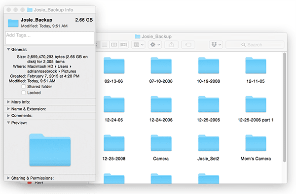
Figure 4: Inside the “Josie_Backup” directory I have a number of images, some of which have been imported into iPhoto and others which have not. My goal is to determine which subdirectories of photos inside “Josie_Backup” need to be added to “Masters”.
The
Josie_Backupdirectory contains a number of photos of my dog (Josie) along with numerous unrelated family photos.
My goal is to determine which directories and images have already been imported into iPhoto and which directories I still need to import into iPhoto and organize.
Using image hashing we can make quick work of this project.
Understanding perceptual image hashing and difference hashing
The image hashing algorithm we will be implementing for this blog post is called difference hashing or simply dHash for short.
I first remember reading about dHash on the HackerFactor blog during the end of my undergraduate/early graduate school career.
My goal here today is to:
- Supply additional insight to the dHash perceptual hashing algorithm.
- Equip you with a hand-coded dHash implementation.
- Provide a real-world example of image hashing applied to an actual dataset.
The dHash algorithm is only four steps and is fairly straightforward and easy to understand.
Step #1: Convert to grayscale
Figure 5: The first step in image hashing via the difference hashing algorithm is to convert the input image (left) to grayscale (right).
The first step in our image hashing algorithm is to convert the input image to grayscale and discard any color information.
Discarding color enables us to:
- Hash the image faster since we only have to examine one channel
- Match images that are identical but have slightly altered color spaces (since color information has been removed)
If, for whatever reason, you are especially interested in color you can run the hashing algorithm on each channel independently and then combine at the end (although this will result in a 3x larger hash).
Step #2: Resize
Figure 6: The next step in perceptual hashing is to resize the image to a fixed size, ignoring aspect ratio. For many hashing algorithms, resizing is the slowest step. Note: Instead of resizing to 9×8 pixels I resized to 257×256 so we could more easily visualize the hashing algorithm.
Now that our input image has been converted to grayscale, we need to squash it down to 9×8 pixels, ignoring the aspect ratio. For most images + datasets, the resizing/interpolation step is the slowest part of the algorithm.
However, by now you probably have two questions:
- Why are we ignoring the aspect ratio of the image during the resize?
- Why 9×8 — this seems a like an “odd” size to resize to?
To answer the first question:
We squash the image down to 9×8 and ignore aspect ratio to ensure that the resulting image hash will match similar photos regardless of their initial spatial dimensions.
The second question requires a bit more explanation and will be fully answered in the next step.
Step #3: Compute the difference
Our end goal is to compute a 64-bit hash — since 8×8 = 64 we’re pretty close to this goal.
So, why in the world would we resize to 9×8?
Well, keep in mind the name of the algorithm we are implementing: difference hash.
The difference hash algorithm works by computing the difference (i.e., relative gradients) between adjacent pixels.
If we take an input image with 9 pixels per row and compute the difference between adjacent column pixels, we end up with 8 differences. Eight rows of eight differences (i.e., 8×8) is 64 which will become our 64-bit hash.
In practice we don’t actually have to compute the difference — we can apply a “greater than” test (or “less than”, it doesn’t really matter as long as the same operation is consistently used, as we’ll see in Step #4 below).
If this point is confusing, no worries, it will all become clear once we start actually looking at some code.
Step #4: Build the hash
Figure 6: Here I have included the binary difference map used to construct the image hash. Again, I am using a 256×256 image so we can more easily visualize the image hashing algorithm.
The final step is to assign bits and build the resulting hash. To accomplish this, we use a simple binary test.
Given a difference image D and corresponding set of pixels P, we apply the following test: P[x] > P[x + 1] = 1 else 0.
In this case, we are testing if the left pixel is brighter than the right pixel. If the left pixel is brighter we set the output value to one. Otherwise, if the left pixel is darker we set the output value to zero.
The output of this operation can be seen in Figure 6 above (where I have resized the visualization to 256×256 pixels to make it easier to see). If we pretend this difference map is instead 8×8 pixels the output of this test produces a set of 64 binary values which are then combined into a single 64-bit integer (i.e., the actual image hash).
Benefits of dHash
There are multiple benefits of using difference hashing (dHash), but the primary ones include:
- Our image hash won’t change if the aspect ratio of our input image changes (since we ignore the aspect ratio).
- Adjusting brightness or contrast will either (1) not change our hash value or (2) only change it slightly, ensuring that the hashes will lie close together.
- Difference hashing is extremely fast.
Comparing difference hashes
Typically we use the Hamming distance to compare hashes. The Hamming distance measures the number of bits in two hashes that are different.
Two hashes with a Hamming distance of zero implies that the two hashes are identical (since there are no differing bits) and that the two images are identical/perceptually similar as well.
Dr. Neal Krawetz of HackerFactor suggests that hashes with differences > 10 bits are most likely different while Hamming distances between 1 and 10 are potentially a variation of the same image. In practice you may need to tune these thresholds for your own applications and corresponding datasets.
For the purposes of this blog post we’ll only be examining if hashes are identical. I will leave optimizing the search to compute Hamming differences for a future tutorial here on PyImageSearch.
Implementing image hashing with OpenCV and Python
My implementation of image hashing and difference hashing is inspired by the imagehash library on GitHub, but tweaked to (1) use OpenCV instead of PIL and (2) correctly (in my opinion) utilize the full 64-bit hash rather than compressing it.
We’ll be using image hashing rather than cryptographic hashes (such as md5, sha-1, etc.) due to the fact that some images in my needle or haystack piles may have been slightly altered, including potential JPEG artifacts.
Because of this, we need to rely on our perceptual hashing algorithm that can handle these slight variations to the input images.
To get started, make sure you have installed my imutils package, a series of convenience functions to make working with OpenCV easier (and make sure you access your Python virtual environment, assuming you are using one):
$ workon cv
$ pip install imutils
From there, open up a new file, name it
hash_and_search.py, and we’ll get coding:
# import the necessary packages
from imutils import paths
import argparse
import time
import sys
import cv2
import os
Lines 2-7 handle importing our required Python packages. Make sure you have
imutilsinstalled to have access to the
pathssubmodule.
From there, let’s define the
dhashfunction which will contain our difference hashing implementation:
def dhash(image, hashSize=8):
        # resize the input image, adding a single column (width) so we
        # can compute the horizontal gradient
        resized = cv2.resize(image, (hashSize + 1, hashSize))

        # compute the (relative) horizontal gradient between adjacent
        # column pixels
        diff = resized[:, 1:] > resized[:, :-1]

        # convert the difference image to a hash
        return sum([2 ** i for (i, v) in enumerate(diff.flatten()) if v])
Our
dhashfunction requires an input
imagealong with an optional
hashSize. We set
hashSize=8to indicate that our output hash will be 8 x 8 = 64-bits.
Line 12 resizes our input
imagedown to
(hashSize + 1, hashSize)— this accomplishes Step #2 of our algorithm.
Given the
resizedimage we can compute the binary
diffon Line 16, which tests if adjacent pixels are brighter or darker (Step #3).
Finally, Line 19 builds the hash by converting the boolean values into a 64-bit integer (Step #4).
The resulting integer is then returned to the calling function.
Now that our
dhashfunction has been defined, let’s move on to parsing our command line arguments:
# construct the argument parse and parse the arguments
ap = argparse.ArgumentParser()
ap.add_argument("-a", "--haystack", required=True,
        help="dataset of images to search through (i.e., the haytack)")
ap.add_argument("-n", "--needles", required=True,
        help="set of images we are searching for (i.e., needles)")
args = vars(ap.parse_args())
Our script requires two command line arguments:
-
--haystack
: The path to the input directory of images that we will be checking the--needles
path for. -
--needles
: The set of images that we are searching for.
Our goal is to determine whether each image in
--needlesexists in
--haystackor not.
Let’s go ahead and load the
--haystackand
--needlesimage paths now:
# grab the paths to both the haystack and needle images
print("[INFO] computing hashes for haystack...")
haystackPaths = list(paths.list_images(args["haystack"]))
needlePaths = list(paths.list_images(args["needles"]))

# remove the `` character from any filenames containing a space
# (assuming you're executing the code on a Unix machine)
if sys.platform != "win32":
        haystackPaths = [p.replace("\\", "") for p in haystackPaths]
        needlePaths = [p.replace("\\", "") for p in needlePaths]
Lines 31 and 32 grab paths to the respective images in each directory.
When implementing this script, a number of images in my dataset had spaces in their filenames. On normal Unix systems we escape a space in a filename with a
\, thereby turning the filename
Photo 001.jpginto
Photo\ 001.jpg.
However, Python assumes the paths are un-escaped so we must remove any occurrences of
\in the paths (Lines 37 and 38).
Note: The Windows operating system uses
\to separate paths while Unix systems uses
/. Windows systems will naturally have a
\in the path, hence why I make this check on Line 36. I have not tested this code on Windows though — this is just my “best guess” on how it should be handled in Windows. User beware.
# grab the base subdirectories for the needle paths, initialize the
# dictionary that will map the image hash to corresponding image,
# hashes, then start the timer
BASE_PATHS = set([p.split(os.path.sep)[-2] for p in needlePaths])
haystack = {}
start = time.time()
Line 43 grabs the subdirectory names inside
needlePaths— I need these subdirectory names to determine which folders have already been added to the haystack and which subdirectories I still need to examine.
Line 44 then initializes
haystack, a dictionary that will map image hashes to respective filenames.
We are now ready to extract image hashes for our
haystackPaths:
# loop over the haystack paths
for p in haystackPaths:
        # load the image from disk
        image = cv2.imread(p)

        # if the image is None then we could not load it from disk (so
        # skip it)
        if image is None:
                continue

        # convert the image to grayscale and compute the hash
        image = cv2.cvtColor(image, cv2.COLOR_BGR2GRAY)
        imageHash = dhash(image)

        # update the haystack dictionary
        l = haystack.get(imageHash, [])
        l.append(p)
        haystack[imageHash] = l
On Line 48 we are loop over all image paths in
haystackPaths.
For each image we load it from disk (Line 50) and check to see if the image is
None(Lines 54 and 55). If the
imageis
Nonethen the image could not be properly read from disk, likely due to an issue with the image encoding (a phenomenon you can read more about here), so we skip the image.
Lines 58 and 59 compute the
imageHashwhile Lines 62-64 maintain a list of file paths that map to the same hash value.
The next code block shows a bit of diagnostic information on the hashing process:
# show timing for hashing haystack images, then start computing the
# hashes for needle images
print("[INFO] processed {} images in {:.2f} seconds".format(
        len(haystack), time.time() - start))
print("[INFO] computing hashes for needles...")
We can then move on to extracting the hash values from our
needlePaths:
# loop over the needle paths
for p in needlePaths:
        # load the image from disk
        image = cv2.imread(p)

        # if the image is None then we could not load it from disk (so
        # skip it)
        if image is None:
                continue

        # convert the image to grayscale and compute the hash
        image = cv2.cvtColor(image, cv2.COLOR_BGR2GRAY)
        imageHash = dhash(image)

        # grab all image paths that match the hash
        matchedPaths = haystack.get(imageHash, [])

        # loop over all matched paths
        for matchedPath in matchedPaths:
                # extract the subdirectory from the image path
                b = p.split(os.path.sep)[-2]

                # if the subdirectory exists in the base path for the needle
                # images, remove it
                if b in BASE_PATHS:
                        BASE_PATHS.remove(b)
The general flow of this code block is near identical to the one above:
- We load the image from disk (while ensuring it’s not
None
) - Convert the image to grayscale
- And compute the image hash
The difference is that we are no longer storing the hash value in
haystack.
Instead, we now check the
haystackdictionary to see if there are any image paths that have the same hash value (Line 87).
If there are images with the same hash value, then I know I have already manually examined this particular subdirectory of images and added them to iPhoto. Since I have already manually examined it, there is no need for me to examine it again; therefore, I can loop over all
matchedPathsand remove them from
BASE_PATHS(Lines 89-97).
Simply put: all images + associated subdirectores in
matchedPathsare already in my iPhotos album.
Our final code block loops over all remaining subdirectories in
BASE_PATHSand lets me know which ones I still need to manually investigate and add to iPhoto:
# display directories to check
print("[INFO] check the following directories...")

# loop over each subdirectory and display it
for b in BASE_PATHS:
        print("[INFO] {}".format(b))
Our image hashing implementation is now complete!
Let’s move on to applying our image hashing algorithm to solve my needle/haystack problem I have been trying to solve.
Image hashing with OpenCV and Python results
To see our image hashing algorithm in action, scroll down to the “Downloads” section of this tutorial and then download the source code + example image dataset.
I have not included my personal iPhotos dataset here, as:
- The entire dataset is ~39GB
- There are many personal photos that I do not wish to share
Instead, I have included sample images from the UKBench dataset that you can play with.
To determine which directories (i.e., “needles”) I still need to examine and later add to the “haystack”, I opened up a terminal and executed the following command:
$ python hash_and_search.py --haystack haystack --needles needles
[INFO] computing hashes for haystack...
[INFO] processed 7466 images in 1111.63 seconds
[INFO] computing hashes for needles...
[INFO] check the following directories...
[INFO] MY_PIX
[INFO] 12-25-2006 part 1
As you can see from the output, the entire hashing and searching process took ~18 minutes.
I then have a nice clear output of the directories I still need to examine: out of the 14 potential subdirectories, I still need to sort through two of them,
MY_PIXand
12-25-2006 part 1, respectively.
By going through these subdirectories I can complete my photo organizing project.
As I mentioned above, I am not including my personal photo archive in the “Downloads” of this post. If you execute the
hash_and_search.pyscript on the examples I provide in the Downloads, your results will look like this:
$ python hash_and_search.py --haystack haystack --needles needles
[INFO] computing hashes for haystack...
[INFO] processed 1000 images in 7.43 seconds
[INFO] computing hashes for needles...
[INFO] check the following directories...
[INFO] PIX
[INFO] December2014
Which effectively demonstrates the script accomplishing the same task.
Where can I learn more about image hashing?
If you’re interested in learning more about image hashing, I would suggest you first take a look at the imagehashing GitHub repo, a popular (PIL-based) Python library used for perceptual image hashing. This library includes a number of image hashing implementations, including difference hashing, average hashing, and others.
From there, take a look at the blog of Tham Ngap Wei (a PyImageSearch Gurus member) who has written extensively about image hashing and even contributed a C++ image hashing module to the OpenCV-contrib library.
Summary
In today’s blog post we discussed image hashing, perceptual hashing, and how these algorithms can be used to (quickly) determine if the visual contents of an image are identical or similar.
From there, we implemented difference hashing, a common perceptual hashing algorithm that is (1) extremely fast while (2) being quite accurate.
After implementing difference hashing in Python we applied it to a real-world dataset to solve an actual problem I was working on.
I hope you enjoyed today’s post!
To be notified when future computer vision tutorials are published here on PyImageSearch, be sure to enter your email address in the form below!
Downloads:
The post Image hashing with OpenCV and Python appeared first on PyImageSearch.
from PyImageSearch http://ift.tt/2A9hjsg
via IFTTT
1 comment:
nice bLog! its interesting. thank you for sharing.... 统计作业代写
Post a Comment